The idea: when no line fits, find the closest one
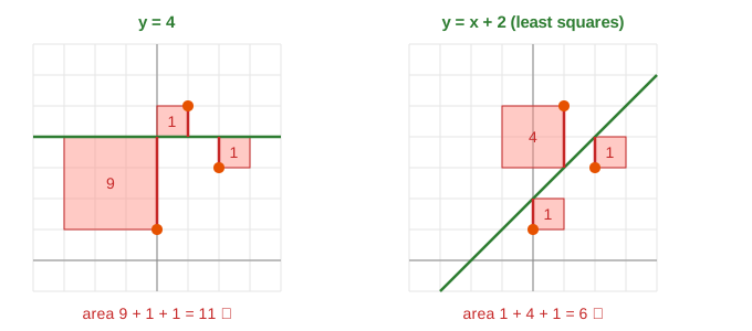
Three points (0, 1), (1, 5), (2, 3) do not lie on one line. Least squares picks the line y = mx + c that misses them by the least, where the miss is measured as the sum of the squared residuals. The page draws each squared residual as a real square, so the quantity being minimised is a total area you can see. The answer here is y = x + 2, with squares 1 + 4 + 1 = 6.
Three equations, two unknowns
A line through all three points would need m·xᵢ + c = yᵢ for each point. In matrix form that is Ax = b:
The first column of A holds the x values, the second is all ones. Three equations and two unknowns make an overdetermined system. The first two rows force c = 1 and m = 4, and then the third row says 2·4 + 1 = 9, not 3. The line y = x + 1 through points 1 and 3 misses point 2 by 3 instead: every line misses something (Demo: 3 points, no exact fit).
Minimising the squares
For any guess (m, c) the residual of point i is eᵢ = yᵢ − (mxᵢ + c), the red vertical segment from the point to the line. Least squares minimises e₁² + e₂² + e₃² = ‖b − Ax‖². Squaring makes every miss count as positive, and it makes the total a smooth bowl in (m, c) with a single lowest point. Start from y = 4 (area 11) and move the line toward the best one in four equal steps: the area falls 11 → 8.81 → 7.25 → 6.31 → 6 (Demo: squares shrink to the best line).
The column space picture
Put the three y values into one vector b = (1, 5, 3) in 3D. Every guess gives Ax = m·a₁ + c·a₂, a combination of the two columns a₁ = (0, 1, 2) and a₂ = (1, 1, 1). All such combinations form a plane through the origin, the column space C(A). Ax = b has no solution because b is not on that plane. ‖b − Ax‖ is the distance from b to the point Ax, so least squares asks for the point of the plane closest to b. That point is the foot of the perpendicular from b: the projection p = (2, 3, 4) (Demo: projection of b onto C(A)).
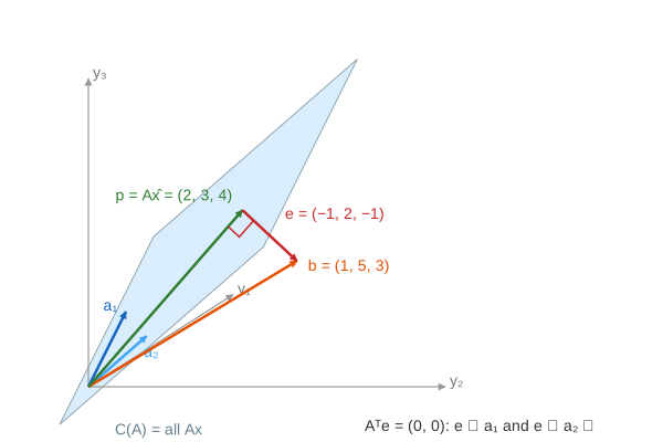
The canvas draws 3D with a simple oblique projection (y₁ goes down-left), so right angles in space do not look exactly square on the screen. The numbers in the panel check them.
The normal equations
e = b − Ax̂ is perpendicular to the plane, so it is perpendicular to both columns: a₁·e = 0 and a₂·e = 0. Together that is Aᵀ(b − Ax̂) = 0, or
These are the normal equations ("normal" means perpendicular). AᵀA is a small 2×2 matrix of sums, and Aᵀb collects Σxy and Σy:
| step | numbers |
|---|---|
| AᵀA, Aᵀb | [5 3; 3 3], (11, 9) |
| equations | (1) 5m + 3c = 11, (2) 3m + 3c = 9 |
| (1) − (2) | 2m = 2, so m = 1 |
| back substitute in (2) | 3 + 3c = 9, so c = 2 |
| check | e = (−1, 2, −1), Aᵀe = (0, 0) |
Subtracting one equation from the other is one step of Gaussian elimination (Demo: normal equations AᵀA x̂ = Aᵀb). The projection itself is p = A(AᵀA)⁻¹Aᵀb, the same idea as projecting one vector onto another in vectors and the dot product, but onto a plane instead of a line. With three points the plane leaves only one perpendicular direction, (1, −2, 1), so every best residual is a multiple of it.
Outliers
Squares grow fast: one miss of 6 costs 36, while six misses of 1 cost only 6. Move point 2 from y = 5 to y = 8 and the old line y = x + 2 costs 1 + 25 + 1 = 27. The new least-squares line is y = x + 3, cost 4 + 16 + 4 = 24: the whole line moves up by 1, and the two good points now miss by 2 each to take some of the load off point 2 (Demo: an outlier pulls the line). That is why least squares is sensitive to outliers; robust fits use absolute values or cap the penalty.
Exact solve vs gradient descent
The normal equations give the answer in one solve. Linear regression by gradient descent minimises the same mean squared error by small downhill steps instead; that scales to millions of features and to models with no closed form, such as logistic regression. Both land on the same line for a straight-line fit.
See also L1 vs L2 Regularization: ridge adds λI to the normal equations; lasso drives weights to exactly 0.
What the page leaves out
Only three points and a straight line are used. With n points A is n×2 and the same formulas hold; with polynomial or several features A just gets more columns. In practice AᵀA is not formed directly when it is badly conditioned: QR decomposition or the SVD (the pseudoinverse) solve the problem more accurately. Weighted least squares, regularisation (ridge regression adds λI to AᵀA), the statistics of the fit (R², standard errors) and total least squares, which measures perpendicular rather than vertical distance, are not shown.