The idea: make the residuals small
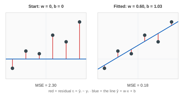
Linear regression predicts a number from a feature with a straight line, ŷ = w·x + b. The weight w is the slope and the bias b is where the line crosses x = 0. For each training point the residual rᵢ = ŷᵢ − yᵢ is how far the line misses it: on the canvas, the red segment from the point to the line. The mean squared error MSE = (1/n)·Σ rᵢ² is one number for how bad the whole line is. Fitting means finding the w and b with the smallest MSE.
One gradient descent step
The page starts with w = 0 and b = 0 and improves them with gradient descent. The gradient of the MSE is an average over the points of each residual:
- ∂L/∂w = (2/n)·Σ rᵢ·xᵢ
- ∂L/∂b = (2/n)·Σ rᵢ
Points above the line (rᵢ < 0) pull it up, points below push it down, and points far from x = 0 tilt it more. The update goes against the gradient: w ← w − η·∂L/∂w, b ← b − η·∂L/∂b, where η is the learning rate. On the canvas each Step shows the residuals, the gradient box flying from the gradient rows to w and b, and then the line moving. The table lists every point's x, y, ŷ and r. (Demo 1)
The normal equation
For linear regression the minimum can also be computed directly. Write each point as a row [xᵢ 1] of a matrix X; setting the gradient to zero gives the normal equation XᵀX·θ = Xᵀy, so θ = (w, b) = (XᵀX)⁻¹·Xᵀy. On the 8 clean points XᵀX = [[42, 0], [0, 8]] and the answer is w* ≈ 0.576, b* ≈ 0.994 — the green line. After about 20 gradient steps the blue line sits on it. The closed form costs a d×d matrix inverse (d = number of features), so with millions of features or rows gradient descent is cheaper.
Outliers pull the line
Because the residuals are squared, a point 6 units away costs 36 times as much as a point 1 unit away. Adding one outlier at (3, −4) to the clean data drags the least-squares slope from about 0.58 down to about 0.22 (and b from 0.99 to 0.37). (Demo 2) Losses that grow more slowly for large errors — absolute error or the Huber loss — are less sensitive to outliers.
Learning rate too high
The MSE is a bowl in (w, b). Along its steepest direction it curves with strength λmax = 2·mean(xᵢ²) = 10.5 here, and a step multiplies the distance to the minimum along it by 1 − η·λmax. With η = 0.1 that is −0.05 (fine); with η = 0.25 it is −1.625: every step lands on the other side, further away, and w and b blow up. So η must stay below 2/λmax ≈ 0.19. (Demo 3) Centering and scaling the features keeps λmax small and the bowl round; that is why the page's x values are centred on 0. See Gradient Descent for the loss surface itself.
Logistic regression: a probability instead of a number
For a yes/no label y ∈ {0, 1}, logistic regression keeps the same w·x + b but squashes it with the sigmoid σ(z) = 1 / (1 + e^−z) into a probability p = P(y = 1 | x). The loss is log loss (cross-entropy): −(1/n)·Σ [yᵢ·ln pᵢ + (1 − yᵢ)·ln(1 − pᵢ)]. A confident wrong answer costs a lot: p = 0.01 for a class-1 point costs ln 100 ≈ 4.6. Its gradient has the same shape as before, with pᵢ − yᵢ in place of the residual: ∂L/∂w = (1/n)·Σ (pᵢ − yᵢ)·xᵢ, ∂L/∂b = (1/n)·Σ (pᵢ − yᵢ).
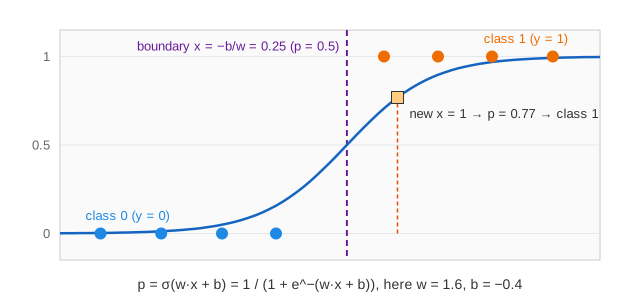
The decision boundary is where p = 0.5, i.e. w·x + b = 0, at x = −b/w. A new point gets a probability from the curve and a class by comparing it with 0.5 (Demo 5). There is no closed form: the unknowns sit inside σ, so logistic regression is always fitted iteratively (gradient descent, or Newton's method, which is what most libraries use).
Separable data and regularization
When a boundary separates the two classes perfectly, the loss keeps falling as w grows: a steeper sigmoid gives every point a probability closer to its label. The weights grow forever and the loss only reaches 0 at infinity. (Demo 4) One mislabeled point makes the classes overlap and gives a finite best w. In practice L2 regularization (adding λ·w² to the loss) keeps the weights finite either way.
| Linear regression | Logistic regression | |
|---|---|---|
| predicts | a number ŷ = w·x + b | a probability p = σ(w·x + b) |
| loss | mean squared error | log loss (cross-entropy) |
| gradient term per point | 2·rᵢ, rᵢ = ŷᵢ − yᵢ | pᵢ − yᵢ |
| closed form | yes: (XᵀX)⁻¹·Xᵀy | no |
| sensitive to | outliers (squared error) | separable data (w grows without bound) |
See also Gradient Descent for learning rates and momentum, Perceptron for a linear classifier with a hard step instead of a sigmoid, Neural Network for many logistic units stacked in layers, and Backpropagation for how their gradients are computed.
The normal equation is a linear system; see Gaussian Elimination for how such a system is solved.
The same straight-line fit solved exactly in one step, with the normal equations and the projection picture, in least squares as projection.
See also L1 vs L2 Regularization: lasso and ridge penalties on the weights, side by side.
See Logistic Regression for the two-input version: the boundary as a line in the plane, p = 0.1 / 0.9 lines, and per-point log loss bars.
See also Support Vector Machine: the same kind of linear boundary, chosen by the widest margin with the hinge loss instead of log loss.
When a straight line is too simple or a high-degree polynomial too flexible, see Bias–Variance Trade-off and Cross-Validation.
A fitted slope describes how variables move together in the data, not what changing one would cause; see Simpson's paradox and confounders.
Before fitting a line, Correlation and Scatter Plots shows how Pearson r measures how close the points are to one, and how an outlier or a curve misleads it.
For what the slope m and the intercept b of a line y = mx + b mean on their own, see Linear Functions: Slope and Intercept.
What the page leaves out
Only one feature is used, so the fit is a line in a 2-D plot; with d features it is a hyperplane and w is a vector, and logistic regression's boundary becomes a line or plane between the classes. Steps use all points (full batch); stochastic and mini-batch gradient descent, feature scaling, regularization, Newton's method, multi-class softmax regression and evaluating on held-out data are only described.