The idea: simplify the equations without changing the answer
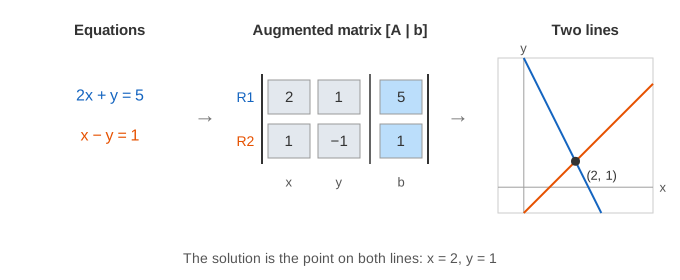
A linear system is a set of equations like 2x + y = 5 and x − y = 1. Write only the numbers and you get the augmented matrix [A | b]: one row per equation, the coefficients of x, y, z on the left of the bar and the right-hand sides on the right. Gaussian elimination changes the rows step by step until the answer can be read off, using only moves that keep the set of solutions the same.
The three row operations
| Operation | Written | Why the solutions stay the same |
|---|---|---|
| swap two rows | R2 ↔ R3 | the same equations in another order |
| scale a row by k ≠ 0 | R2 ← (−2/3)·R2 | both sides of one equation multiplied by the same number |
| add a multiple of another row | R2 ← R2 − (1/2)·R1 | a point that solves R1 and R2 also solves R2 − m·R1, and the step can be undone |
Every step on the canvas is one of these. The new row is computed entry by entry: a copy of −m·R1 flies onto R2 and is added to it. All numbers are kept as exact fractions (1/2, −3/2), so nothing is rounded.
Forward elimination and pivots
Go column by column. The first non-zero entry in the current row of that column is the pivot (orange). For every row below, the multiplier is m = entry / pivot, and Rk ← Rk − m·Rpivot turns that entry into 0. Then move one row down and one column right. When no column is left the matrix is in row-echelon form: the pivots make a staircase and everything below them is 0. (Demo 2: 2x + y − z = 8, −3x − y + 2z = −11, −2x + y + 2z = −3.)
Back substitution
The last pivot row now has a single unknown, so it gives its value directly. Put that value into the rows above, which removes that unknown from them, and repeat upwards. The page does this with row operations too: divide each pivot row by its pivot so the pivot is 1, then clear the entries above it. The matrix ends in reduced row-echelon form, the identity on the left and the solution on the right (Demo 2 ends at x = 2, y = 3, z = −1). Clearing above and below every pivot like this is also called Gauss–Jordan elimination.
What the row operations do to the lines
With two unknowns each row a·x + b·y = c is a line. Adding a multiple of R1 to R2 replaces line 2 with another line through the same crossing point, because the crossing point satisfies both old rows and so satisfies any combination of them. In Demo 1 R2 becomes −(3/2)y = −3/2, a horizontal line y = 1, and at the end R1 is the vertical line x = 2. Scaling a row does not move its line at all.
Zero pivots and row swaps
If the pivot spot holds 0, no multiple of that row can clear anything below it. Look further down the column for a non-zero entry and swap that row up (Demo 3: after the first column R2 is [0, 0, 1 | 3], so R2 ↔ R3). If the whole rest of the column is 0, that column has no pivot and its unknown is a free variable. Computer libraries swap even when the pivot is only small, choosing the largest entry in the column (partial pivoting), because dividing by a tiny pivot blows up rounding errors in floating point.
One, none or infinitely many solutions
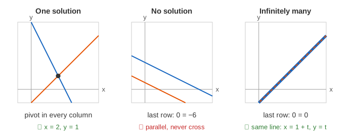
The echelon form tells which case you are in. A row 0 = c with c ≠ 0 means no solution: the equations contradict each other (Demo 4: x + 2y = 4 and 2x + 4y = 2, parallel lines, R2 becomes 0 = −6). A row 0 = 0 with fewer pivots than unknowns means infinitely many solutions: each free variable becomes a parameter t (Demo 5: x − y = 1 twice over, so x = 1 + t, y = t). A pivot in every column means exactly one solution.
Cost and the determinant
Clearing one column of an n × n matrix touches about n² entries, so elimination takes about n³/3 multiply-adds, which is O(n³). The same elimination gives the determinant: the product of the pivots, with the sign flipped once per row swap. A zero determinant is exactly the case where some column has no pivot. See Determinant for that view, Eigenvectors for another use of matrices, and Linear Regression, whose normal equation is a linear system solved this way.
When a system has more equations than unknowns and no solution, least squares solves the 2×2 normal equations instead.
Circuit simulators solve the node equations G·v = i of a resistor network this way; see Ohm's Law and Kirchhoff's Laws for where those equations come from.
What the page leaves out
Only small square systems (2×2 and 3×3) with integer inputs are shown, and swaps happen only for a zero pivot. Partial pivoting, rounding error, LU decomposition (keeping the multipliers to solve many right-hand sides), non-square systems, and the 3-D picture of three planes meeting at a point are only described.