LU Decomposition: Elimination Saved as L times U

The idea: keep the multipliers

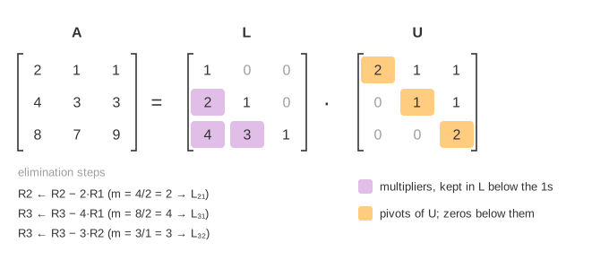
Gaussian elimination clears the entries below each pivot with steps like R2 ← R2 − 2·R1. The number 2 is the multiplier m = entry / pivot. Run elimination on A alone and it ends in an upper-triangular matrix U. Write each multiplier into a lower-triangular matrix L, at the same row and column it cleared, with 1s on the diagonal. Then A = L·U: that is the LU decomposition.

Why L·U gives back A

Each row of U is the row of A minus the multiples of the rows above that elimination subtracted. Add them back and you get A: row 3 of A = 4·(row 1 of U) + 3·(row 2 of U) + (row 3 of U). Those coefficients 4, 3, 1 are exactly row 3 of L. The check panel on the canvas does this sum for every row. (Demo 1: A = [2 1; 1 −1], one multiplier 1/2, U = [2 1; 0 −3/2].)

In matrix language each step is an elimination matrix E, and E₃₂E₃₁E₂₁A = U. Undoing the steps in reverse order gives A = E₂₁⁻¹E₃₁⁻¹E₃₂⁻¹U, and that product of inverses is L, with the multipliers simply sitting in their places.

Solving Ax = b with two triangular solves

Since A = LU, the equation Ax = b is L(Ux) = b. Call y = Ux and solve in two easy passes:

Pass	Equation	Order	Why it is easy
forward substitution	Ly = b	top down	row 1 of L is [1 0 0], so y₁ = b₁; each next row has one new unknown
back substitution	Ux = y	bottom up	the last row of U has one unknown; divide by its pivot and move up

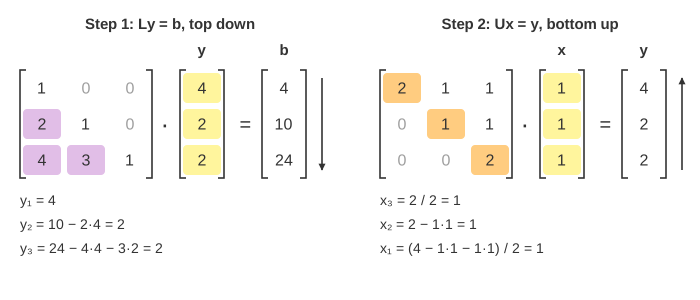
Forward substitution is the elimination applied to b, done afterwards: y is exactly the right-hand side that Gaussian elimination on [A | b] would have produced. (Demo 2: y = (8, 1, 1), then x = (2, 3, −1).)

Factor once, solve many

Elimination is the expensive part, and it only looks at A. Once L and U are stored, every new b costs just the two triangular solves. (Demo 3: the second b reuses L and U and goes straight to Ly = b.)

n	factor A (about n³/3 multiply-adds)	one solve with L and U (about n²)
3	9	9
100	333,333	10,000
1,000	333 million	1 million

For a 3×3 matrix the two are the same size; for a big one, re-solving is hundreds of times cheaper. This is why solvers factor once, and why computing the inverse matrix to solve a system is not needed: x = A⁻¹b costs the same n² per b but A⁻¹ costs more to build than L and U.

Zero pivots: PA = LU

If a pivot spot holds 0, a lower row with a non-zero entry is swapped up. The swap is recorded in a permutation matrix P, and the multipliers already stored in L for those two rows move with them. The result is PA = LU: L and U factor A with its rows reordered. To solve, b gets the same swap first, then LUx = Pb. (Demo 4: after column 1, row 2 of U is [0, 0, 1], so R2 ↔ R3.) Libraries swap even when the pivot is only small, picking the largest entry in the column (partial pivoting), to keep rounding errors small.

The determinant comes free

det L = 1 and det U is the product of its diagonal, so det A = ± (product of the pivots), with the sign flipped once per row swap. Demo 2: 2 · (1/2) · (−1) = −1. See Determinant for what that number means.

In practice: LAPACK's getrf computes PA = LU and getrs does the two triangular solves; SciPy exposes them as lu_factor and lu_solve, and MATLAB's backslash uses them for square systems. L and U are stored together in one n × n array, since the 1s on L's diagonal need no storage.

What the page leaves out

Only small invertible matrices with exact fractions are shown, and rows are swapped only for a zero pivot. Partial pivoting by size, rounding error and stability, singular matrices (a 0 left on U's diagonal), the Cholesky factorization A = LLᵀ for symmetric positive-definite matrices, LDU, and blocked or sparse LU are only described or not covered.

References

Gilbert Strang — Introduction to Linear Algebra, section 2.6: Elimination = Factorization: A = LU

MIT OpenCourseWare 18.06 Linear Algebra — lecture 4: factorization into A = LU

SciPy — scipy.linalg.lu_factor and lu_solve

Wikipedia — LU decomposition