The idea: the columns are where î and ĵ land
A linear transformation of the plane is a map that keeps grid lines straight, parallel and evenly spaced, and keeps the origin where it is. Every vector is a mix of the two basis vectors î = (1, 0) and ĵ = (0, 1): (x, y) = x·î + y·ĵ. A linear map keeps that mix, so it is fixed by just two arrows: where î lands and where ĵ lands. Write them as the columns of a 2×2 matrix and you have the whole map.
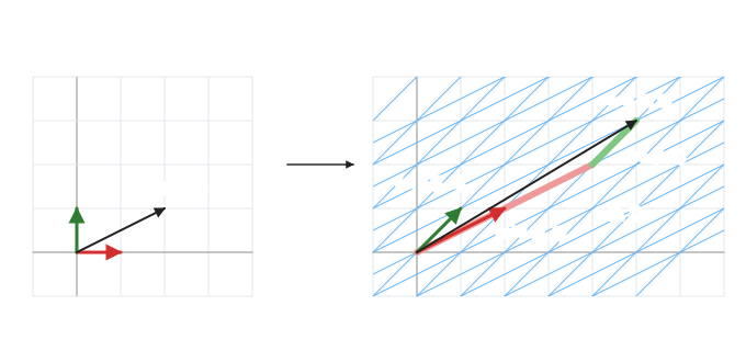
On the canvas the grey grid stays put and is the ruler. The blue grid, the red arrow (where î lands) and the green arrow (where ĵ lands) move with the matrix. The info panel on the right shows the matrix with column 1 in red and column 2 in green (Demo: where î and ĵ go).
Each of the basic transforms has its own page: rotation, reflection, scaling, shear and projection. Each one shows its matrix, what it keeps (lengths, angles, area), its determinant, its eigenvectors and its inverse.
More on the same idea: squeeze mapping, composing transforms, affine transforms and homogeneous coordinates, the inverse by row reduction, diagonalization, column space and null space and Gram–Schmidt and QR. In 3D: rotation, reflection, projection, shear, quaternions and perspective projection.
Matrix times vector is a walk
To find where v = (x, y) lands, use the same recipe on the new arrows: walk x copies of column 1, then y copies of column 2. With A = [2 1; 1 1] and v = 2î + 1ĵ, the walk is 2·(2, 1) + 1·(1, 1) = (5, 3) (Demo: v = 2î + 1ĵ mapped). On the blue grid the black arrow still reads (2, 1); on the grey grid it reads (5, 3). The row-by-row rule you learn in school computes the same thing:
Doing one map after another is again a linear map, so it has a matrix too: its columns are where the first map sends î and ĵ, pushed through the second. That is matrix multiplication, see Matrix Multiplication.
Change of basis: one point, two sets of coordinates
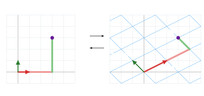
Any two non-parallel vectors b1, b2 form a basis: every point is c1·b1 + c2·b2 in exactly one way, and (c1, c2) are its B-coordinates [p]B. Put b1 and b2 as the columns of P. Then P turns B-coordinates into standard ones, and P−1 turns standard coordinates into B-coordinates:
With b1 = (2, 1) and b2 = (−1, 1), the point p = (3, 3) is 2·b1 + 1·b2, so [p]B = (2, 1). P = [2 −1; 1 1], det P = 3, P−1 = (1/3)[1 1; −1 2], and P−1·(3, 3) = (1/3)·(6, 3) = (2, 1). On the canvas the b-grid is drawn by applying P; then P−1 straightens it and the arrow that ended at p ends at (2, 1) (Demo: change of basis (P and P⁻¹)).
Where this shows up: a camera or robot frame (Changing Coordinates in 2D), and diagonalisation, where the basis is made of eigenvectors so the map becomes plain stretching along each axis.
The inverse undoes the map
If no two points land on the same spot, the map can be run backwards. The inverse A−1 sends column 1 back to î and column 2 back to ĵ, so A−1A = I. For a 2×2 matrix: swap a and d, negate b and c, and divide by the determinant ad − bc.
For A = [2 1; 1 1], det = 1 and A−1 = [1 −1; −1 2]. Check: A−1·(5, 3) = (5 − 3, −5 + 6) = (2, 1). On the canvas the blue grid morphs back onto the grey one and the black arrow returns from (5, 3) to (2, 1) (Demo: the inverse undoes A).
Singular matrices: span, null space, no inverse
When the two columns are parallel, every x·(col 1) + y·(col 2) lies on one line. With S = [2 1; 2 1] the columns are (2, 2) and (1, 1), so the whole plane is squashed onto the line y = x. That line is the span of the columns (the column space); it has dimension 1, so the rank of S is 1.
A whole line of inputs lands on 0: S·(1, −2) = 1·(2, 2) − 2·(1, 1) = (0, 0), and so does every multiple t·(1, −2). That line is the null space. Different inputs collide too: u = (1, 0) and w = (0, 2) both land on (2, 2), because w − u = (−1, 2) is in the null space. No map can send (2, 2) back to both, so S has no inverse, and the formula agrees: det S = 0 and 1/0 is undefined (Demo: singular, no inverse (null space)).
| Matrix | Columns | det | Image | Null space | Inverse |
|---|---|---|---|---|---|
| [2 1; 1 1] | (2, 1), (1, 1) | 1 | the whole plane | only 0 | [1 −1; −1 2] |
| [2 −1; 1 1] | (2, 1), (−1, 1) | 3 | the whole plane | only 0 | (1/3)[1 1; −1 2] |
| [2 1; 2 1] | (2, 2), (1, 1) | 0 | the line y = x | the line through (1, −2) | none |
Rank + dimension of the null space = 2 here (1 + 1), the number of columns. For a system Sx = b this means: no solution when b is off the line, and a whole line of solutions when it is on it. See also Gaussian Elimination and Rotation and Scaling in 2D.
What the page leaves out
Only 2×2 matrices with small whole-number entries are drawn, so the grid stays inside the panel. Translations (which move the origin and are not linear; computer graphics adds them with 3×3 homogeneous matrices), 3D and n-dimensional maps, non-square matrices, similar matrices P−1AP (the same map written in another basis), and how inverses are computed in practice (row reduction or LU, never the adjugate formula for big matrices) are not shown.