The idea: weighted sums and a bend, layer after layer
A feed-forward neural network turns a list of numbers into another list of numbers. It is built from neurons, and every neuron does the same two things: it adds up its inputs, each multiplied by a weight, plus a bias; then it passes that sum through an activation function. Neurons are grouped in layers, and each layer's outputs are the next layer's inputs. Running an input through all layers is the forward pass.
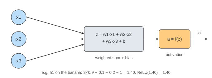
The page uses a network with 3 inputs, 4 hidden neurons and 3 outputs. It classifies a fruit from three features between 0 and 1: x1 = how long it is, x2 = how red, x3 = how orange. The outputs are the classes banana, apple and orange. The weights are fixed, as if the network was already trained; how they are learned is Backpropagation.
One neuron
Hidden neuron h1 has weights (3, −1, −1) and bias −1. For the banana, x = (0.9, 0.1, 0.2):
z1 = 3×0.9 + (−1)×0.1 + (−1)×0.2 + (−1) = 1.40
a1 = ReLU(1.40) = max(0, 1.40) = 1.40
Large positive weight on "long", negative weights on the colours: h1 is a "long thing" detector. h2 and h3 detect red and orange, h4 fires for colourful round fruit. Nobody tells a real network what its neurons should detect; training finds whatever helps. (Demo 1: full forward pass)
A layer is a matrix product
Put each hidden neuron's weights in one row and the layer becomes one formula: z = W·x + b, then a = f(z) element by element. W1 is 4×3 (4 neurons, 3 inputs), so the shapes are (4×3)·(3×1) + (4×1) = (4×1). The output layer is z = W2·a + b2 with W2 3×4. Libraries and GPUs compute layers this way, often for a whole batch of inputs at once (X·Wᵀ for a matrix X of inputs). (Demo 2: matrix view)
Activation functions
| activation | f(z) | range | used where |
|---|---|---|---|
| ReLU | max(0, z) | [0, ∞) | the default in hidden layers; cheap, exact zeros |
| sigmoid | 1 / (1 + e−z) | (0, 1) | older hidden layers; a single yes/no output; LSTM gates |
| tanh | (ez − e−z) / (ez + e−z) | (−1, 1) | RNNs; zero-centred, unlike sigmoid |
| none | z | all reals | output layers before softmax (logits), regression outputs |
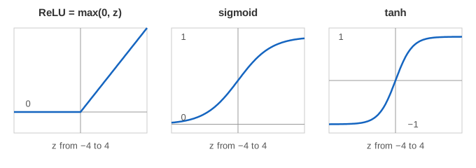
Changing the activation changes everything after it. The peach (0.3, 0.6, 0.7) is red and orange at once. With ReLU the network says orange 74.3%; with sigmoid, whose hidden outputs are never exactly 0, it is unsure (orange 52.9%, apple 40.0%); with tanh, orange 71.6%. (Demo 3: change activation)
Softmax: from scores to probabilities
The output neurons have no activation. Their values, the logits, can be any real number. Softmax turns them into probabilities: pk = ezk / Σj ezj. Every p is positive and they add up to 1; the largest logit gets the largest share, and a gap of 1 in logits means a factor e ≈ 2.7 in probability. For the banana the logits (3.30, −1.40, −1.40) become (0.982, 0.009, 0.009). Implementations subtract the largest logit first so ez cannot overflow; the result is the same. Training compares p with the true class using cross-entropy loss.
Dead ReLUs
A ReLU outputs 0 whenever z ≤ 0. That is normal for some inputs: h2 and h3 are 0 for the banana. But if z ≤ 0 for every input, the neuron always outputs 0 and its slope is always 0, so backpropagation never changes its weights: it is dead. Set b4 = −3 and h4 is 0 for all four fruits; the network still works with three neurons, but h4 is wasted. A too-large learning rate can kill many ReLUs at once; Leaky ReLU (a small slope for z < 0) avoids it. (Demo 4: dead ReLU)
Why the activation matters
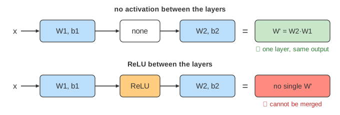
Without an activation the network is z = W2(W1·x + b1) + b2 = (W2·W1)·x + (W2·b1 + b2). Multiply the two matrices once and you have a single layer W' (3×3) and b' that give exactly the same logits for every input. Any stack of linear layers is one linear layer: it can only draw straight boundaries, so it can never solve XOR (see Perceptron). With ReLU, sigmoid or tanh in between, there is no such W': the bend is what lets more layers learn more. (Demo 5: no activation, Demo 6: with ReLU)
From here to bigger networks
Real networks are the same forward pass with bigger matrices: thousands of inputs, many layers, millions or billions of weights. A classic first step up is a network that reads handwritten digits from 784 pixels: see Neural Network: Recognizing Handwritten Digits. Image networks use convolution layers that share weights across positions; sequence models use RNNs and LSTMs or attention. Inside every transformer block of a large language model there is exactly this kind of two-layer MLP, and the model's last layer is a softmax over the vocabulary. The weights all come from training with backpropagation and gradient descent.
To see how the softmax output is trained, with the cross-entropy loss, its gradient p − y and the max-subtracted stable form, see Softmax & Cross-Entropy.
The layer's W·x is a matrix product, worked cell by cell in Matrix Multiplication.
See also CNN vs Transformer, two ways a network mixes the patches of an image.
A diffusion model trains a network to predict the noise added to data, then runs it backwards to generate new samples: see Diffusion Model.
See also Dropout & Batch Normalization: two layers that sit between these dense layers and behave differently in training and at inference.
What the page leaves out
Training (see Backpropagation), loss functions beyond a mention of cross-entropy, batches, weight initialization, normalization layers, dropout, residual connections and other activations (GELU, Leaky ReLU, softplus) are not shown. The weights are hand-picked round numbers, not the result of training.