The idea: the widest street
A support vector machine (SVM) is a classifier for two classes, + and −. Like the perceptron, it draws a line f(x) = w·x + b = 0 and predicts + on one side and − on the other. The difference is which line. Many lines separate two clusters; the perceptron stops at the first one that works. The SVM picks the line with the widest empty street around it: the band between f(x) = −1 and f(x) = +1 with no point inside. Half the street's width is the margin, the distance from the line to the closest point.
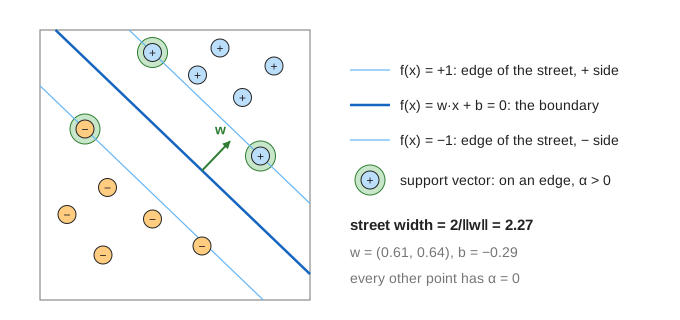
A point far from the line is a safe call; a point close to it could flip with a little noise. Making the closest distance as large as possible gives the line that is most robust, and in theory it also generalizes best. (Demo 1: many lines, one widest street: Try Lines shows three separating lines and the distance d of each one's closest point; the SVM line beats them all.)
Margin = 2/‖w‖
Scale w and b so that the closest points have f(x) = ±1 exactly. A point x at f(x) = 1 is at distance 1/‖w‖ from the line, so the street is 2/‖w‖ wide. A wide street means a short w. Training is therefore:
minimize   ½‖w‖²
subject to y·(w·x + b) ≥ 1   for every point (y = +1 or −1)
This is a convex quadratic program: one best answer, no local minima, unlike gradient training of a neural network. On the two clusters the answer is w = (0.61, 0.64), b = −0.29, a street 2.27 wide.
Support vectors
Solvers work on the dual problem: one weight α ≥ 0 per point, and w = Σ α·y·x. At the optimum almost all α are 0. The points with α > 0 are the support vectors: they lie on the edges of the street (or inside it, see below). Only they define the line. Remove any other point and the answer stays the same, exactly; remove a support vector and the line moves. (Demo 2: only support vectors matter: dropping the far point (−1.6, −2) changes nothing; dropping the support vector (−2, 0.8) tilts the line and widens the street from 2.27 to 2.39.)
The page solves the dual with SMO (sequential minimal optimization): it repeatedly picks the two α that break the optimality conditions the most and solves for that pair exactly, the method LIBSVM uses.
Soft margin and C
Real data has noise: one odd point can force a very narrow street, and with overlapping classes no street exists at all. The soft margin lets point i violate the street by a slack ξi = max(0, 1 − y·f(x)) and charges for it:
minimize ½‖w‖² + C·Σ ξi
ξ between 0 and 1 means inside the street but on the right side; ξ > 1 means on the wrong side. C sets the price of slack. In the dual it caps every α at C.
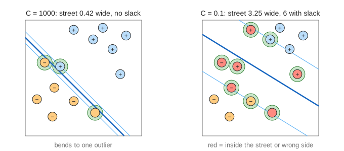
| clusters + outlier, linear | street width | support vectors | points with slack |
|---|---|---|---|
| C = 1000 (hard margin) | 0.42 | 3 | 0 |
| C = 1 | 2.34 | 4 | 2 |
| C = 0.1 | 3.25 | 8 | 6 |
Large C trusts every point and overfits the outlier; small C trusts the overall shape. In practice C is picked by cross-validation. (Demo 3: soft margin, C = 1000 vs 0.1)
The kernel trick
On the ring data the + points sit inside a circle of − points. No line separates them; the solver's best linear answer is w = 0, predicting − everywhere (Demo 4: ring, no line works). The fix is to give each point a new coordinate. With φ(x) = (x1, x2, x1² + x2²), the third coordinate is the squared distance from the origin: inner points stay low and outer points rise up a bowl. In that lifted space a flat plane z = 3.06 separates them, and back in the plane the boundary x1² + x2² = 3.06 is a circle of radius 1.75 (Demo 5: kernel trick lifts the ring).
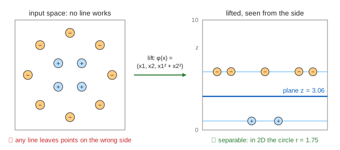
The dual problem only ever uses dot products φ(xi)·φ(xj). A kernel K(xi, xj) computes that dot product directly, without building φ(x): the polynomial kernel (xi·xj + 1)^d covers all products of up to d coordinates, and the RBF kernel exp(−γ‖xi − xj‖²) corresponds to an infinite-dimensional φ. The page builds φ explicitly (three features) so that w can be shown.
SVM, perceptron, logistic regression
| model | which line | loss | output |
|---|---|---|---|
| perceptron | the first that separates | update on mistakes only | a class |
| logistic regression | most likely under a sigmoid model | log loss, every point counts | a probability |
| SVM | the widest street | hinge loss max(0, 1 − y·f(x)) + ½‖w‖²/C | a class (and a distance) |
See also The Perceptron (the line that stops at the first fit), Logistic Regression, K-Nearest Neighbors and Gradient Descent.
What the page leaves out
Only two inputs and one explicit lift; real SVMs use kernels such as RBF without ever computing φ, and scale the features first. The page does not show how b is computed in detail, multi-class SVMs (one-vs-rest, one-vs-one), support vector regression, probability outputs (Platt scaling), or choosing C and γ by cross-validation. C = 1000 stands in for a true hard margin.