Train a Tiny Network on Your Points

The idea: straight lines, bent together

Click in the plot to add points. Each point is blue (class y = 1) or orange (y = 0). A small neural network learns to tell them apart. It has two inputs, the point's coordinates x₁ and x₂. It has one hidden layer of H neurons (1 to 4) and one output neuron. The output a is a number between 0 and 1: near 1 means "blue", near 0 means "orange". The background of the plot shows a for every spot, so you see the decision boundary a = 0.5 move while the network trains. Everything runs in your browser, in plain JavaScript. This is a small version of the TensorFlow Playground.

The key picture: each hidden neuron draws one straight line (dashed on the plot). The output neuron adds the hidden neurons up. So the boundary is made of pieces of those lines, bent where they meet. One line can split two blobs. It takes two or more lines to cut out the XOR pattern, and three to fence in a circle.

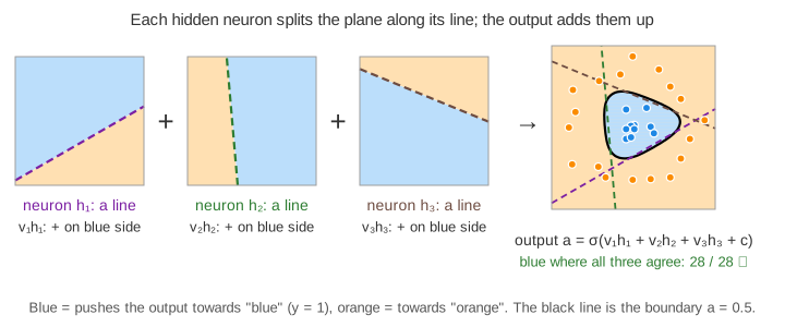
One neuron is one line

A hidden neuron j has two weights w_j1, w_j2 and a bias b_j. It computes a weighted sum, then squeezes it with tanh:

zj = wj1·x1 + wj2·x2 + bj
hj = tanh(zj)                     (between −1 and 1; tanh(0) = 0)

The points where z_j = 0 form a straight line, w_j1x₁ + w_j2x₂ + b_j = 0. On one side z_j > 0 and h_j is positive; on the other side it is negative. The small arrow on each dashed line points to the positive side. Far from the line h_j is close to +1 or −1; near it, h_j changes smoothly. So a hidden neuron answers one question: "which side of my line is this point on, and how far?" That is all a single neuron can do, which is why one neuron can never learn XOR. The Perceptron page shows the same line for a neuron with a hard step instead of tanh.

The output adds the lines up

The output neuron has one weight v_j per hidden neuron and a bias c. It uses the sigmoid σ, so its answer is between 0 and 1:

z = v1·h1 + v2·h2 + … + vH·hH + c
a = σ(z) = 1 / (1 + e^(−z))         (a > 0.5 means blue)

z is a weighted sum of the H "ramps" h_j. With H = 1 the output is blue on one side of one line: the boundary is that line (Demo 1: two blobs, H = 1 is enough, 20 of 20 points after 200 epochs). With H = 2, the sum of two ramps can be high in a band between two lines and low outside. That is exactly XOR's shape (Demo 2). With H = 3, three ramps that all point inwards add up to a high value only inside their triangle (Demo 3). The corners come out rounded, because each tanh is smooth.

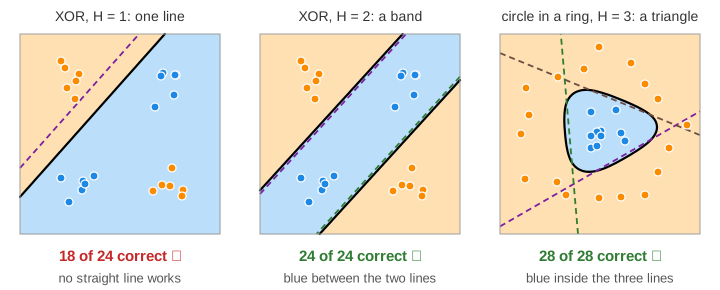
The numbers from the demos:

Data	H	After training	Why
two blobs (20 points)	1	20 / 20 ✓	one line separates them
XOR (24 points)	1	18 / 24 ✗ (75 %), C stuck at 0.49	no line separates XOR; the best line gets 3 of the 4 clusters
XOR (24 points)	3	24 / 24 ✓	a band between two lines
circle in a ring (28 points)	2	23 / 28 ✗	two lines cannot close a region
circle in a ring (28 points)	3	28 / 28 ✓	a triangle around the circle

Adding neurons only allows a better boundary; training still has to find it. On XOR, H = 2 is enough in principle, but from some random starts gradient descent gets stuck at 12 to 14 of 24. With H = 3 or 4 there are spare lines, and every start we tried at η = 1 reached 24 of 24. This idea goes much further: with enough hidden neurons, one hidden layer can approximate any continuous function (see Nielsen's chapter 4 in the references).

Why tanh in the hidden layer, σ at the output

The hidden layer uses tanh because it is centred on 0: a hidden neuron says −1 on one side of its line and +1 on the other, and exactly 0 on the line. Its slope at 0 is 1, four times the sigmoid's 0.25, so the gradients that reach the hidden layer are larger and training is faster. The TensorFlow Playground uses tanh by default too. The output uses the sigmoid because its answer should be a number between 0 and 1 that can be read as "how sure it is blue".

The cost: binary cross-entropy

To learn, the network needs one number that says how wrong it is. For a point with class y and answer a, the binary cross-entropy is:

Cp = −[ y·ln a + (1 − y)·ln(1 − a) ]      = −ln a for blue,  −ln(1 − a) for orange
C  = (1/N) · Σp Cp                         (the average over all N points)

A right and sure answer costs almost 0 (−ln 0.99 = 0.01). A wrong and sure answer costs a lot (−ln 0.01 = 4.6). An answer of a = 0.5 costs ln 2 = 0.693, which is why a fresh network starts near 0.69. We pick cross-entropy rather than squared error because, together with the sigmoid, it makes the output's error simply δ = a − y (next section). With squared error the error gets an extra factor a(1 − a), which is almost 0 when the network is sure. So a network that is sure and wrong would learn very slowly.

Backpropagation in a 2 → H → 1 network

Step runs one epoch with every number shown. It follows one point P (the one with the black ring; click a point to choose it). Backpropagation uses the chain rule to find ∂C/∂w for every weight. The useful middle value is each neuron's error δ = ∂C/∂z. For one point:

output:    δ   = ∂C/∂a · σ'(z) = (a − y)/(a(1 − a)) · a(1 − a) = a − y
hidden j:  δj  = δ · vj · tanh'(zj) = δ · vj · (1 − hj²)
weights:   ∂C/∂vj  = δ · hj        ∂C/∂c  = δ
           ∂C/∂wj1 = δj · x1       ∂C/∂wj2 = δj · x2       ∂C/∂bj = δj

Read the second line as a path: weight w_j1 changes z_j, which changes h_j, which changes z through v_j, which changes a, which changes C. The chain rule multiplies the local slope of each link. On the canvas, δ·v_j flies back from the output to each hidden neuron. A hidden neuron far from its line (h ≈ ±1) has 1 − h² ≈ 0, so it hardly learns: it is saturated. The page computes these derivatives exactly; a check against finite differences, (C(w + ε) − C(w − ε)) / 2ε, agrees to about 10⁻⁹. For a network with more layers, see Backpropagation and Draw a Digit.

One step of gradient descent

The same backpropagation runs for every point, and the derivatives are averaged: that average is the gradient ∇C. It points where C rises fastest, so every weight and bias takes a small step the other way:

w ← w − η · ∂C/∂w          (η: the learning rate; 1 on this page unless you change it)

One such step over all the points is an epoch. This is full-batch gradient descent: every epoch uses every point, so it is deterministic. Train runs 200 epochs and shows them in four steps. Watch each dashed line slide and turn as its w_j1, w_j2, b_j change, and the cost curve fall. With 4 hidden neurons the network has 4·3 + 4 + 1 = 17 numbers to learn. See Gradient Descent for the step itself on a cost surface.

A worked example with numbers

Take one hidden neuron (H = 1) with w₁₁ = 1, w₁₂ = −1, b₁ = 0, output weight v₁ = 2 and c = −0.5. Take one blue point P = (0.5, 0.2), so y = 1.

1. Forward: z₁ = 1·0.5 − 1·0.2 + 0 = 0.3, h₁ = tanh 0.3 = 0.291. Then z = 2·0.291 − 0.5 = 0.083 and a = σ(0.083) = 0.521. Just above 0.5: blue, but barely.
2. Cost: C = −ln 0.521 = 0.653.
3. Output error: δ = a − y = 0.521 − 1 = −0.479. Negative, so z should go up. ∂C/∂v₁ = δ·h₁ = −0.140 and ∂C/∂c = −0.479.
4. Hidden error: δ₁ = δ·v₁·(1 − h₁²) = −0.479 · 2 · 0.915 = −0.877. Then ∂C/∂w₁₁ = δ₁·0.5 = −0.439, ∂C/∂w₁₂ = δ₁·0.2 = −0.175 and ∂C/∂b₁ = −0.877.
5. Update with η = 1: w₁₁ = 1.439, w₁₂ = −0.825, b₁ = 0.877, v₁ = 2.140, c = −0.021.
6. Forward again: z₁ = 1.432, h₁ = 0.892, a = σ(1.888) = 0.869. The cost fell from 0.653 to 0.141.

Every derivative was negative here, so every number went up: the network moved its line so that P sits deeper on the blue side.

The learning rate

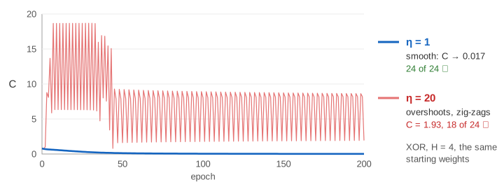
η sets the step size. Too small and training is slow. Too large and each step jumps across the valley of C instead of going down into it. In Demo 4: learning rate too large, XOR with η = 20 starts at C = 0.79, is at 8.8 by the third epoch, and then jumps up and down: between 0.7 and 18.7 in the first 50 epochs, between 1.7 and 9.1 later. After 200 epochs only 18 of 24 points are right (C = 1.93). The big steps also push hidden neurons far from their lines, where 1 − h² ≈ 0, and those neurons stop learning. The same start with η = 1 falls smoothly to C = 0.017 and 24 of 24.

Overfitting: bending around mislabeled points

Real data has mistakes. Demo 5: mislabeled points, overfitting uses two blobs with one blue point placed among the orange ones and one orange point among the blue ones. After 200 epochs the boundary is almost straight: 28 of 30 correct, and the two odd points are left on the wrong side. That is the sensible answer. Train 2,000 more epochs with H = 4 and the network bends its boundary around both of them: 30 of 30 and C = 0.008. The training points are now all right, but the boundary has curls that come from two mistakes, not from the real pattern. A new point near them would be put in the wrong class. This is overfitting: a network with enough neurons can fit noise. Real training keeps some points aside (a validation set) and stops when the error on those stops falling, or penalises large weights (regularisation).

What the page leaves out

Real networks train on mini-batches or single examples (stochastic gradient descent) and use optimisers such as Adam instead of the plain step. Hidden layers usually use ReLU, and there are many layers, not one. The page has no test set, no regularisation and no input features beyond x₁, x₂ (the Playground can also feed x₁², sin x₁ and so on). Weights start uniformly in fixed ranges from a fixed seed, so that every demo is repeatable. For a trained network that reads handwritten digits, see Draw a Digit; for the forward pass of a larger network with softmax, see Neural Network Forward Pass.

References

Daniel Smilkov, Shan Carter — TensorFlow Playground

Michael Nielsen — Neural Networks and Deep Learning, ch. 4: A visual proof that neural nets can compute any function

3Blue1Brown — But what is a neural network? (Deep Learning, chapter 1)

Michael Nielsen — Neural Networks and Deep Learning, ch. 3: the cross-entropy cost function