The idea: two layers that act differently in training and at inference
Most layers of a neural network compute the same thing every time. Dropout and batch normalization do not: during training they use randomness or the other examples in the mini-batch, and at inference they switch to a fixed, deterministic rule. In PyTorch the switch is model.train() / model.eval(); the page's Mode select is that switch.
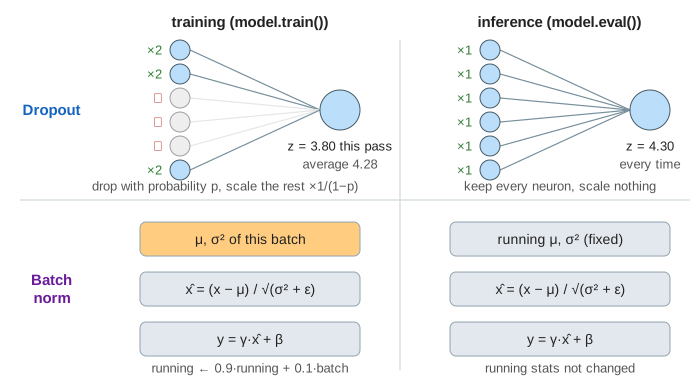
The left lane follows one example's hidden layer of 6 ReLU outputs h (sum 4.30) into the next neuron, z = Σ h̃, with every weight 1 so the sums stay readable. The right lane follows a batch-norm layer over 3 features a, b, c, whose values come from a seeded random stream with true means 4, −2, 0.5 and variances 4, 1, 0.25.
Dropout: drop at random, scale the rest
On every training pass each neuron's output is set to 0 with probability p (here 0.5, the nn.Dropout default). A new random mask is drawn on every pass, so the network can never rely on one particular neuron being there. The page draws the mask from a seeded generator so every demo replays the same: the first pass drops n3, n4 and n5.
Modern libraries use inverted dropout: the kept outputs are multiplied by 1/(1−p) (×2 here). A neuron is kept with probability 1−p, so its expected output is (1−p)·h/(1−p) = h, the same as with no dropout. One pass can be far off (3.80 on the first pass, 7.00 on another), but the average over 20 passes is 4.28, close to 4.30 (Demo: dropout — 20 training passes, then inference).
training:   h̃ᵢ = h · mᵢ / (1 − p)      mᵢ = 0 with probability p, else 1
inference:  h̃ᵢ = h                     (dropout is the identity)
At inference dropout does nothing: every neuron is kept and nothing is scaled, so the next neuron gets 4.30 every time, the same scale it saw on average during training.
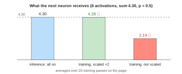
Forget the scaling and training sends only (1−p) of the sum on average: 2.14 against 4.30 at inference, twice as big as anything the next layer was trained on (Demo: dropout without the 1/(1−p) scaling). The original 2014 paper did it the other way round: no scaling in training, and every weight multiplied by 1−p at inference. Both give the same expected values; inverted dropout keeps the inference code unchanged.
Why it helps: each pass trains a different thinned network that shares weights with all the others, and inference approximately averages that huge ensemble. Neurons cannot co-adapt to fix each other's mistakes, so they learn more robust features. It is a regularizer, like the weight penalties in L1 vs L2 regularization; usual values are p = 0.1–0.5, larger on big fully connected layers.
Batch normalization: normalize each feature over the batch
A batch normalization layer looks at one mini-batch of B examples. For each feature (column) separately it computes the batch mean μ and variance σ², normalizes, and then applies a learned scale γ and shift β:
μ  = (1/B) Σ xᵢ            σ² = (1/B) Σ (xᵢ − μ)²
x̂ᵢ = (xᵢ − μ) / √(σ² + ε)   ε = 1e-5
yᵢ = γ · x̂ᵢ + β
After normalization every feature has mean 0 and variance 1 in the batch, whatever its scale was: feature a (spread out around 2.28) and feature b (bunched up around −1.53) end up on the same footing. γ and β are learned by gradient descent like any weight, so the network can still choose another mean and spread; on the page they are fixed at γ = 1, 2, 1 and β = 0, 1, 0, so feature b comes out with mean 1 and variance 4 (Demo: batch norm — one training step).
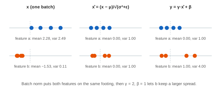
Normalized inputs keep each layer's activations in a steady range while the weights below it change, which allows larger learning rates and makes deep networks much easier to train. The batch statistics also add a little noise, a mild regularizing effect.
Running statistics: what inference uses
At inference there may be just one example, and its prediction must not depend on which other examples happen to share its batch. So during training the layer also keeps running estimates, updated after every batch with momentum = 0.1 (PyTorch's default):
running_mean = 0.9 · running_mean + 0.1 · μ
running_var  = 0.9 · running_var  + 0.1 · σ² · B/(B − 1)     (unbiased variance)
They start at 0 and 1. At inference the layer uses them as fixed numbers and does not update them. After 30 training batches they are 3.67, −1.97, 0.50 and 4.01, 1.05, 0.26, close to the true values, and inference outputs stay in the normal range (Demo: batch norm — 30 batches, then inference). After only 2 batches the running mean is still 0.63, −0.34, 0.10, so inference puts x̂ as far out as 5.64 (Demo: batch norm — inference after only 2 batches): the network sees inputs on a scale it was never trained on.
Pitfalls
- Forgetting
model.eval()at inference: dropout keeps dropping neurons, so predictions are random, and batch norm normalizes with the batch of test examples, so a prediction depends on its neighbours. - Tiny batches. With B = 1 the mean is the example itself and σ² = 0, so x̂ = 0 and y = β: all information is gone. PyTorch refuses it in training ("Expected more than 1 value per channel when training") (Demo: batch norm — a batch of 1). Batches of 2–8 work but give noisy statistics; layer normalization (normalize over the features of one example) avoids the problem and is what Transformers use.
- Train/test mismatch from running statistics that have not settled, or that were computed on data that looks different from the test data.
Side by side
| Dropout | Batch normalization | |
|---|---|---|
| Training | random mask, keep with probability 1−p, scale by 1/(1−p) | normalize with the batch's μ, σ², then γ·x̂ + β; update running stats |
| Inference | identity: nothing dropped, nothing scaled | normalize with the running μ, σ²; nothing updated |
| Learned parameters | none (p is a hyperparameter) | γ and β per feature |
| Depends on other examples | no | yes, in training |
| Main purpose | regularization (less overfitting) | stable, faster training; some regularization |
See also Neural Network (Forward Pass) for the layers these sit between, and L1 vs L2 Regularization for weight penalties, the other classic way to fight overfitting.
What the page leaves out
The backward pass: gradients flow only through kept neurons in dropout, and batch norm's gradient also passes through μ and σ². γ and β stay fixed instead of being learned. Convolutional batch norm (BatchNorm2d) computes one μ and σ² per channel over the batch and all pixels. The page also leaves out layer, group and instance normalization, dropout variants (DropConnect, spatial dropout, Monte Carlo dropout that keeps dropout on at inference to estimate uncertainty), and the debate over whether batch norm helps by reducing "internal covariate shift" or by smoothing the loss surface.