The idea: destroy the data with noise, then learn to undo it
A diffusion model generates new data by learning to remove noise. During training it takes real data and buries it under Gaussian noise in many small steps: the forward process. A neural network learns to undo one small step at a time. To generate, it starts from pure noise and runs the steps backwards: the reverse process. Image generators such as Stable Diffusion and DALL·E 2 work this way on millions of pixels; this page does the same thing on points in 2D, so you can watch every point move.
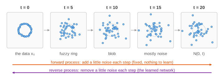
On the canvas the data is the ring of radius 1: 40 training points x₀ lie on it. The big plot shows the points, the bars at the top right show how much signal and noise each step t holds, and the panel below them shows one training example.
The forward process and the shortcut
One forward step shrinks every point a little and adds a little Gaussian noise: xₜ = √(1−βₜ)·xₜ₋₁ + √βₜ·z with z ~ N(0, I). The noise schedule β₁ … β_T sets how much noise each step adds. The page uses T = 20 steps and the cosine schedule. After the last step nothing of the ring is left: the points follow the standard normal distribution N(0, I), whatever the data was. (Demo 1: forward, add noise for 20 steps.)
Because every step is Gaussian, many steps add up to one Gaussian. With ᾱₜ = (1−β₁)(1−β₂)…(1−βₜ):
xₜ = √ᾱₜ · x₀ + √(1−ᾱₜ) · ε ε ~ N(0, I)So you can jump from x₀ to any t in one go. ᾱₜ is the share of signal left; it is the blue part of each bar.
| t | ᾱₜ (signal) | 1 − ᾱₜ (noise) | what the ring looks like |
|---|---|---|---|
| 0 | 1.00 | 0.00 | the data |
| 5 | 0.85 | 0.15 | a fuzzy ring |
| 10 | 0.49 | 0.51 | a blob, the hole is almost gone |
| 15 | 0.14 | 0.86 | mostly noise |
| 20 | 0.00 | 1.00 | pure noise N(0, I) |
Training: predict the noise
The network ε_θ(xₜ, t) gets a noisy point and the step number, and must say which noise was added. One training step is:
- Pick a data point x₀ and a random step t.
- Draw noise ε ~ N(0, I) and build xₜ = √ᾱₜ·x₀ + √(1−ᾱₜ)·ε with the shortcut.
- The network predicts ε̂ = ε_θ(xₜ, t).
- Loss = |ε − ε̂|², and one gradient step on the weights (backpropagation).
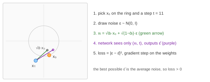
The loss never reaches 0. From xₜ alone the network cannot know exactly where on the ring the point came from, so the best it can do is predict the average noise over all the x₀ that could have produced xₜ. That average is exactly what the reverse process needs. The page does not train a network in the browser: it uses this ideal predictor, x̂₀ = E[x₀ | xₜ], which is what a perfectly trained network would output for the ring. (Demo 2: training, predict the noise that was added.)
Sampling: the reverse loop
x = random point from N(0, I)            // t = T
for t = T, T−1, ..., 1:
    ε̂  = ε_θ(x, t)                       // predict the noise
    x̂₀ = (x − √(1−ᾱₜ)·ε̂) / √ᾱₜ           // where it would have started
    x  = c₁·x̂₀ + c₂·x  +  σₜ·z           // a small step towards x̂₀, plus fresh noise
                                          // (no noise on the last step)
return x
Each step removes only part of the predicted noise and adds back a smaller amount of fresh noise σₜ·z. Early on x̂₀ is a rough guess near the centre; as t falls the guesses sharpen and every point settles on the ring. The samples are new points: none of them is a training point. The orange point leaves a trail so you can follow one sample from noise to data. (Demo 3: generate, 20 denoising steps from noise to the ring.)
Why many small steps
One step from pure noise can only output the average of the data, E[x₀ | noise], and the average of a ring is its centre: every sample lands in the middle, where there is no data at all. This is why one-shot denoising gives blurry images. Small steps let the model commit to a part of the ring a little at a time.
| sampling steps | timesteps visited | samples on the ring (of 40) |
|---|---|---|
| 1 | 20, 0 | 0: all at the centre (Demo 4) |
| 2 | 20, 10, 0 | about 0: they fall inside the ring |
| 5 | 20, 16, 12, 8, 4, 0 | most |
| 20 | every t | all 40 (Demo 3) |
(Demo 5: two steps vs five steps.) Faster samplers such as DDIM and DPM-Solver take bigger steps more cleverly, so real systems need 20–50 network calls instead of the 1 000 steps used in training.
From points to images
For images, x₀ is a whole picture (say 512 × 512 × 3 numbers) instead of 2 numbers, and the network is a large U-Net or transformer that predicts the noise in every pixel. The loop is the same. Text prompts steer it by feeding the text into the network (conditioning) and mixing conditional and unconditional predictions (classifier-free guidance). Stable Diffusion also runs the whole process in a smaller compressed latent space instead of on pixels.
See also the normal distribution, the noise every step adds, and neural networks, the function that learns to predict it.
For two older generative models trained on 2D points, see VAE vs GAN: a variational autoencoder and a generative adversarial network side by side, including mode collapse.
What the page leaves out
The page uses the ideal noise predictor instead of training a real network, and 20 steps instead of the usual 1 000. It leaves out the variational (ELBO) derivation, the score-matching and stochastic-differential-equation view (ε̂ is a scaled score, −√(1−ᾱₜ)·∇log p(xₜ)), learned variances, DDIM's deterministic sampler, conditioning and guidance, latent diffusion, and flow matching.