Diagonalization: A = P D P⁻¹ in Three Moves

The idea: in the right coordinates, a matrix only stretches

Most matrices both turn and stretch the plane, which makes them hard to picture. But many of them have two special directions, the eigenvectors e₁ and e₂, that they only stretch: A·e₁ = λ₁e₁ and A·e₂ = λ₂e₂. Measure every point along those two directions instead of along x and y, and A becomes a plain stretch by λ₁ and λ₂. That is diagonalization: A = P D P⁻¹, where P holds the eigenvectors as columns and D is the diagonal matrix of eigenvalues.

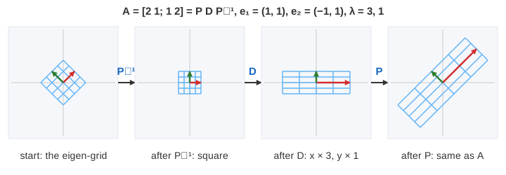
On the canvas the blue grid runs along the eigenvectors (red e₁, green e₂), so it starts slanted. Press A = P D P⁻¹ and the page finds λ₁, λ₂ and e₁, e₂, fills D and P, then plays the three moves one at a time. The grey ghost is the picture under A in one go; the third move lands exactly on it (Demo: A = P D P⁻¹ in three moves).

Eigenvectors are the columns of P, eigenvalues fill D

Put e₁ and e₂ side by side as the columns of P. Then A·P has columns A·e₁ = λ₁e₁ and A·e₂ = λ₂e₂, which is the same as P·D:

$$AP=\left[{\lambda }_1{e}_1{\lambda }_2{e}_2\right]=\left[e_1{e}_2\right]\left[\begin{array}{cc}{\lambda }_1& 0\\ 0& {\lambda }_2\end{array}\right]=PD⟹A=PD{P}^{-1}$$

The last step needs P⁻¹, so e₁ and e₂ must be independent (not on one line). For A = [2 1; 1 2]: det(A − λI) = λ² − 4λ + 3 = (λ − 3)(λ − 1), so λ₁ = 3, λ₂ = 1, with e₁ = (1, 1) and e₂ = (−1, 1). That gives P = [1 −1; 1 1], D = diag(3, 1) and P⁻¹ = ½[1 1; −1 1]. The order must match: column 1 of P goes with the first diagonal entry of D. As checks, λ₁ + λ₂ = trace A and λ₁·λ₂ = det A (the facts panel shows both). A triangular matrix such as [3 1; 0 2] shows its eigenvalues on the diagonal; its P is a shear (Demo: triangular: λ's on the diagonal).

Three moves: P⁻¹, then D, then P

A matrix product acts from right to left, so A·v = P(D(P⁻¹v)). Each factor is a simple move, and P and P⁻¹ are a change of basis:

Move	What it does	For A = [2 1; 1 2]
1. P⁻¹	writes v in eigen-coordinates: e₁ → (1, 0), e₂ → (0, 1)	the diamond grid becomes square
2. D	stretches x by λ₁ and y by λ₂, no turning	x × 3, y × 1
3. P	back to ordinary coordinates: (1, 0) → e₁, (0, 1) → e₂	lands on A·v (the grey ghost)

A negative eigenvalue flips its axis in move 2: for the Fibonacci matrix λ₂ = −1/φ ≈ −0.618, so the y-direction shrinks and turns over.

Powers are easy: Aⁿ = P Dⁿ P⁻¹

Multiply A by itself and the inner P⁻¹P pairs cancel: A² = P D P⁻¹ P D P⁻¹ = P D² P⁻¹, and in general Aⁿ = P Dⁿ P⁻¹. A power of a diagonal matrix is just the powers of its entries, Dⁿ = diag(λ₁ⁿ, λ₂ⁿ). For A = [2 1; 1 2]:

$$A^n=\frac{1}{2}\left[\begin{array}{cc}{3}^n+1& 3^n-1\\ 3^n-1& 3^n+1\end{array}\right],A^{10}=\left[\begin{array}{cc}29525& 29524\\ 29524& 29525\end{array}\right]$$

The page applies A three times one by one, then jumps straight to n = 10 with D¹⁰ = diag(59049, 1) (Demo: powers: A¹⁰ the easy way). The same trick defines functions of a matrix: e^A = P·diag(e^λ₁, e^λ₂)·P⁻¹, which solves systems of linear differential equations.

The dominant eigenvalue wins

Write the start vector in eigen-coordinates, x₀ = c₁e₁ + c₂e₂. Then every power just multiplies each part by its own λ: Aⁿx₀ = c₁λ₁ⁿe₁ + c₂λ₂ⁿe₂. If |λ₁| > |λ₂|, the e₁ part outgrows the other by the factor |λ₁/λ₂|ⁿ, so the direction of Aⁿx₀ swings toward e₁. For [2 1; 1 2] and x₀ = (1, 0) = ½e₁ − ½e₂ the angle to e₁ goes 45°, 18.4°, 6.3°, 2.1°, … The black arrow on the canvas shows only the direction; the table keeps the exact numbers.

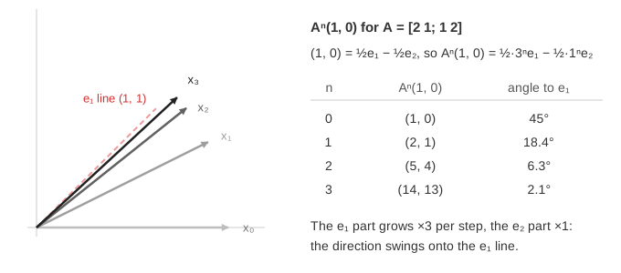
This is power iteration, the simplest way to find the largest eigenvalue (see Eigenvectors), and it is why a Markov chain settles into its stationary distribution: the eigenvalue 1 dominates and every other part dies out. When λ₂ is close to λ₁ the swing is slow; for [3 1; 0 2] the e₂ share only shrinks by ⅔ per step.

Fibonacci and the golden ratio

The matrix A = [1 1; 1 0] turns (F(n), F(n−1)) into (F(n) + F(n−1), F(n)) = (F(n+1), F(n)), so Aⁿ(1, 0) = (F(n+1), F(n)). Its eigenvalues are the roots of λ² − λ − 1 = 0: the golden ratio φ = (1 + √5)/2 ≈ 1.618 and −1/φ ≈ −0.618. Since |φ| wins, F(n+1)/F(n) → φ. Because the losing eigenvalue is negative, the ratios land above and below φ in turn (Demo: Fibonacci and the golden ratio):

n	3	4	5	6	7	8	10
F(n+1)/F(n)	3/2 = 1.5	5/3 ≈ 1.667	8/5 = 1.6	13/8 = 1.625	21/13 ≈ 1.615	34/21 ≈ 1.619	89/55 ≈ 1.618

Diagonalizing gives Binet's formula: x₀ = (1, 0) = (1/√5)(e₁ − e₂), so F(n) = (φⁿ − (−1/φ)ⁿ)/√5. The second term is less than ½ in size, so F(n) is simply φⁿ/√5 rounded to the nearest whole number.

When it fails: the shear and the rotation

Not every matrix can be diagonalized. The shear [1 1; 0 1] has λ = 1 twice, but A − I = [0 1; 0 0] keeps only the x-axis fixed: one line of eigenvectors for a double eigenvalue. Such a matrix is called defective. There is no second column for P; and if there were, D = I would force A = P·I·P⁻¹ = I. Its powers [1 n; 0 1] grow like n instead of λⁿ, and the arrow creeps toward the x-axis slowly (Demo: shear: not diagonalizable). The rotation by 90°, [0 −1; 1 0], keeps no real line at all: λ² + 1 = 0 gives λ = ±i. With complex P = [1 1; −i i] and D = diag(i, −i) the formula still holds, but there is no real picture; the powers go around with period 4 because i⁴ = 1 (Demo: rotation: no real eigenvectors; see Complex Numbers).

A	λ	eigenvectors	diagonalizable?
[2 1; 1 2]	3, 1	(1, 1), (−1, 1)	✓ yes, P can be a rotation (symmetric)
[1 1; 1 0]	φ, −1/φ	(φ, 1), (−1/φ, 1)	✓ yes (symmetric)
[3 1; 0 2]	3, 2	(1, 0), (−1, 1)	✓ yes, two different λ's
[1 1; 0 1]	1, 1	(1, 0) only	✗ no, defective
[0 −1; 1 0]	i, −i	(1, −i), (1, i)	✗ not over ℝ, ✓ over ℂ

Two useful rules: n different eigenvalues always give n independent eigenvectors, so the matrix is diagonalizable; and every symmetric matrix is diagonalizable with perpendicular eigenvectors, so P can be a rotation and P⁻¹ = Pᵀ (the spectral theorem, behind SVD and PCA).

See also Linear Transformations (columns and change of basis), Eigenvectors, Scaling Matrix (what D does), Shear Matrix and Rotation Matrix (the two failures), Matrix Multiplication, Determinant, Inverse Matrix, Composing Transforms, Squeeze Mapping (D = diag(k, 1/k)), Markov Chains and SVD and PCA.

What the page leaves out

Only five 2×2 matrices are drawn. Larger matrices work the same way (P is n×n with the n eigenvectors as columns), but are not shown. The Jordan form, which is the closest a defective matrix gets to diagonal (for the shear it is the shear itself), is not shown, and neither are the real 2×2 rotation-scaling blocks used for complex eigenvalues, how eigenvalues are computed in practice (the QR algorithm rather than the characteristic polynomial), or matrix functions such as e^A beyond the one formula above.

References

Diagonalizable matrix (Wikipedia)

3Blue1Brown, Essence of Linear Algebra: Eigenvectors and eigenvalues

Gilbert Strang, MIT 18.06 Linear Algebra (lecture 22: Diagonalization and powers of A)

Fibonacci sequence: matrix form (Wikipedia)