Residual connections: x + F(x) lets the gradient skip layers

The idea: add the input back

A layer in a plain network replaces its input: h ← F(h). A residual block keeps the input and adds the layer's output to it: h ← h + F(h). The line that carries h around the layer is the skip connection (or shortcut), and F only has to learn the residual, the change to make. He et al. introduced it in ResNet (2015); today it is in almost every deep model, including every transformer layer.

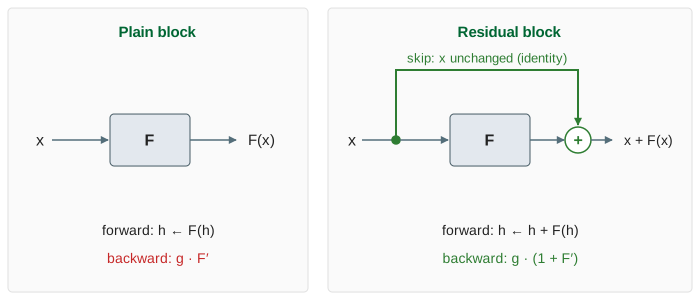
The page builds the same 4, 8 or 12 layers twice, once plain and once with a skip around each layer. To keep the numbers readable each layer is a single number: F_k(h) = a_k · h, with small slopes a = 0.30, −0.20, 0.25, −0.15, … (a sigmoid's slope is never above 0.25, and a freshly initialised layer is also small). The input is x = 1 and the loss sends back ∂L/∂h = 1.

Why a deep plain network stops learning

Backpropagation applies the chain rule layer by layer (see Backpropagation). In a plain stack the gradient that reaches layer k is the product of the slopes of all layers above it:

plain:     ∂L/∂h₀ = a₁ · a₂ · … · aₙ · ∂L/∂hₙ

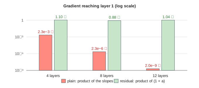
With slopes around 0.2 that product shrinks about 5× per layer. On the page, layer 1 of the 8-layer plain net gets 2.3e−6, and with 12 layers 2.0e−9 (Demo: 12 layers, the plain gradient vanishes). A weight's gradient is this number times the weight's input, so the first layers barely move during training: the vanishing gradient. If the slopes were above 1 the product would blow up instead (exploding gradient). The forward signal fades the same way: the plain net turns x = 1 into 2.3e−6 after 8 layers (Demo: forward pass, 8 layers).

The +1: the gradient takes the skip

The derivative of a residual block is d(h + F(h))/dh = 1 + F′(h). In the animation the gradient splits at each +: one copy goes back along the green skip unchanged, one goes through F and is multiplied by its slope, and the two add at the fork (Demo: backward pass, 8 layers). At layer 8, whose slope is −0.20, that is 1.00 + (−0.20) = 0.80.

residual:  ∂L/∂h₀ = (1 + a₁) · (1 + a₂) · … · (1 + aₙ) · ∂L/∂hₙ

Each factor is close to 1, so the product stays close to 1: layer 1 gets 0.88 with 8 layers and 1.04 with 12. Multiplied out, the product is a sum over all 2ⁿ paths through the network, each path taking either the skip or F at every block. One of those paths is all skips and contributes exactly 1, whatever the layers do.

F = 0: a block that starts as the identity

Set every slope to 0 (Demo: F = 0, a residual block is the identity). The plain net outputs 0 and every gradient is 0: nothing can learn. The residual net outputs x = 1 unchanged and every layer gets gradient 1, so each F starts learning at once. A residual block can always fall back to "do nothing", so adding blocks cannot make the network worse at fitting the training data.

That was the degradation problem ResNet solved: in the paper a 56-layer plain network had a higher training error than a 20-layer one, which is not overfitting but an optimisation failure. With skips, 152 layers trained fine and won ImageNet 2015. Many implementations even initialise the last layer of each block to zero (for example the last batch norm's γ = 0) so every block starts as the identity.

Real blocks and projection shortcuts

In a real ResNet, F is two or three convolutions with batch normalization and ReLU, and the add needs both sides to have the same shape. Where a stage halves the image and doubles the channels, the shortcut becomes a projection W_sx (a 1×1 convolution with stride 2) instead of the plain identity.

ResNet basic block:   y = ReLU( x + BN(conv(ReLU(BN(conv(x))))) )
transformer layer:    x = x + Attention(LayerNorm(x))
                      x = x + MLP(LayerNorm(x))

A transformer is a stack of these two residual updates. The vector x that runs through all of them is called the residual stream: every attention and MLP sublayer reads it and adds its result back. Modern models put the normalization inside the branch (pre-LN) so the skip path itself stays a clean identity from the first layer to the last.

	Plain stack	Residual network
Layer update	h ← F(h)	h ← h + F(h)
Gradient through a layer	× F′	× (1 + F′)
Gradient at layer 1, 12 layers on the page	2.0e−9	1.04
Layer with F = 0	kills the signal and the gradient	identity: passes both through
Extra parameters	none	none (a projection only where shapes change)

See also Neural Network Forward Pass for what one layer computes, Backpropagation for the chain rule step by step, and Batch Norm vs Layer Norm for the normalization that sits inside each block.

What the page leaves out

Each layer here is one number with a fixed slope, so F′ does not depend on h and the gradient does not depend on the forward pass; real layers are matrices with ReLU, and the gradient is a product of Jacobian matrices. Nothing is trained: the page shows one backward pass, not weight updates. It also leaves out bottleneck blocks (1×1, 3×3, 1×1 convolutions), DenseNet's concatenated skips, highway networks with learned gates, the U-Net skips that copy encoder features to the decoder, stochastic depth, and the "ensemble of shallow paths" view of why ResNets work.

References

He, Zhang, Ren & Sun (2015) — Deep Residual Learning for Image Recognition

He et al. (2016) — Identity Mappings in Deep Residual Networks

Veit, Wilber & Belongie (2016) — Residual Networks Behave Like Ensembles of Relatively Shallow Networks

Dive into Deep Learning — Residual Networks (ResNet)