The idea: let a hash decide who sees what, then let statistics decide who won
An A/B test (an online controlled experiment) shows two versions of a page to two random groups of real users at the same time and compares what they do. Group A sees the current version (the control), group B the new one (the treatment). Because the groups are random and run side by side, a difference in behaviour can only come from the change itself or from chance. The statistics on this page tell those two apart.
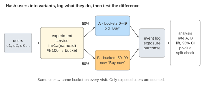
The page runs one experiment, checkout-button: does an orange "Buy now" button sell more than the old blue
"Buy" button? 1,000 users a day open the checkout page. A buys at a true rate of 10%; you pick B's true rate in the bar. The
team running the test never sees those true rates, only the counts. The black tick on each rate bar shows the true rate so
you can see how far the measured rate is from it.
Hash-based assignment
The experiment service does not flip a coin per request. It computes
bucket = fnv1a("checkout-button:" + userId) % 100 and sends buckets 0–49 to A and 50–99 to B. The hash
spreads users evenly and looks random, but it is a pure function, so:
- the same user gets the same variant on every visit, on every server, with nothing stored (Demo 1: u1 comes back and lands in bucket 92 again);
- the experiment name is a salt: another experiment hashes
"other-test:u1"and puts the same user in bucket 24, so experiments don't line up with each other; - ramping is a change of ranges: give B buckets 95–99 for a 5% start, then 50–99 for 50/50, without moving users who are already in B.
Exposures, conversions and the metric
The page logs an exposure event when it actually shows a variant, and a purchase
event when the user buys. The metric is the conversion rate: purchases ÷ unique exposed users, per variant.
Counting unique users matters. In Demo 1 u1 comes back and the log gets a second exposure, but B's n
stays 1. Counting visits would give frequent visitors more weight. Real experiments also watch guardrail
metrics (page latency, errors, refunds) so that a "win" on one number doesn't hide damage elsewhere.
Is the difference real? p-value and confidence interval
Even with no real difference, two groups of 4,000 users won't convert at exactly the same rate. The analysis asks how surprising the observed gap would be if the variants were the same:
| Quantity | Formula | Demo 2 at day 8 |
|---|---|---|
| rates | pA = xA/nA, pB = xB/nB | 391/3,986 = 9.81%, 498/4,014 = 12.41% |
| lift | d = pB − pA | +2.60 points |
| 95% CI | d ± 1.96·√(pA(1−pA)/nA + pB(1−pB)/nB) | [+1.22, +3.97] |
| z (pooled) | d / √(p̂(1−p̂)(1/nA + 1/nB)), p̂ = (xA+xB)/(nA+nB) | 3.70 |
| p-value | chance of a |z| at least this big if A = B | 0.0002 |
The rule fixed before the test: ship B only if p < α = 0.05 at the planned size, which is the same as the
95% CI not containing 0. The CI is the more useful number. It says how big the effect plausibly is, not just whether there
is one. With B at 12%, the test finds the lift (Demo 2). In an A/A test (both at 10%) it
correctly finds nothing, with p = 0.30 at day 8 (Demo 4). An A/A test is how teams check their whole pipeline.
Pick the sample size first
Before the test starts, the team writes down the smallest lift worth detecting, the minimum detectable
effect (MDE). With the baseline rate, α and the power (the chance of detecting the MDE if it
is real, usually 80%), that gives the users needed per variant:
n = 2·(z0.975 + z0.8)²·p̄(1−p̄)/δ².
| Baseline 10%, MDE δ | Users per variant | Days at 1,000 users/day |
|---|---|---|
| 1 point (10% → 11%) | 14,752 | 30 |
| 2 points (10% → 12%) | 3,843 | 8 |
| 3 points (10% → 13%) | 1,776 | 4 |
Halving the effect you want to see costs four times the users. Stopping early wastes the test: after day 1 the same experiment as Demo 2 shows +2.72 points, but the CI is [−0.96, +6.40] and p = 0.15 (Demo 3). That is "not significant", which is not "no effect". Over 1,000 simulated runs, this test detects B's real 2-point lift 82% of the time at day 8, and only 17% of the time after day 1.
Why peeking breaks the test
α = 0.05 means: if you look once, at the planned size, an A/A test comes out "significant" 5% of the time. A dashboard that updates every day invites you to look every day and stop the first time p dips under 0.05. Each look is another chance for noise to cross the line. In Demo 5, an A/A test has p = 0.035 on day 2. Stop there and you ship a "winner" that does nothing. By day 8, p is 0.65.
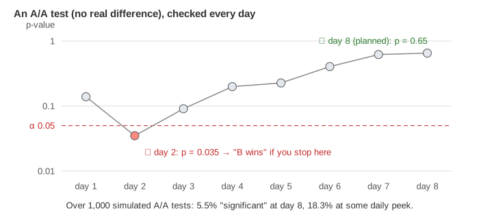
The fixes: decide the size up front and only read the result at the end (as the page does), or use a method built for continuous monitoring: sequential tests (group-sequential boundaries, mSPRT / "always-valid" p-values) that spend α a bit at a time.
Sample ratio mismatch
A 50/50 split will never be exactly 50/50, but it should be close: with 8,000 users, 52/48 is very unlikely by chance. The sample ratio mismatch (SRM) check is a χ² test of nA vs nB against the planned split, and it is read before the conversion numbers. In Demo 6 B is served through a slow redirect. 12% of B's visitors who were not going to buy give up before B's page logs their exposure. B's true rate is the same 10% as A's, but the analysis sees A 3,986 vs B 3,632 (52.3% / 47.7%, χ² p < 0.001), and B looks 1.8 points better with p = 0.011. The lift is fake: B lost its non-buyers. Common real causes are redirects, bot filtering that treats the variants differently, crashes, and logging that fires at a different moment in each variant.
A/B test vs canary release
Both send part of the traffic to something new, but they answer different questions.
| A/B test | Canary release | |
|---|---|---|
| Question | Is B better for users or the business? | Is the new build safe to run? |
| Unit | a user, sticky for weeks | a request (or instance) |
| Split | fixed, often 50/50, for the planned size | small and rising: 1% → 10% → 100% |
| Metric | conversion, revenue, retention | errors, latency, crashes |
| Decision | a statistical test at the end | an alarm, at any time |
See also Canary and Blue/Green Deployments for how traffic is moved between versions, and Naive Bayes for another use of counting and probabilities.
Bayes' Theorem shows why a rare true effect plus a small false-positive rate gives mostly false alarms. See also Central Limit Theorem for why the difference of two conversion rates is close to normal and its error shrinks like 1/√n.
The confidence interval x̄ ± 1.96·σ/√n behind the decision is built step by step, with 20 seeded samples, in Normal Distribution, z-Scores and Confidence Intervals.
See also hypothesis testing with a coin for the p-value, α, type I/II errors and power on a single-sample example.
See Confidence Intervals for what the 95% in a confidence interval does and does not mean.
What the page leaves out
Real experiment platforms also do these things:
- Bayesian A/B tests, which report "the chance that B is better" instead of a p-value;
- multi-armed bandits, which shift traffic toward the winner during the test;
- CUPED and other variance reduction with pre-experiment data, which needs fewer users;
- many metrics and many variants at once, with corrections for multiple testing;
- continuous metrics such as revenue per user (a t-test, heavy tails);
- novelty effects that fade after the first days;
- interference between users, as in marketplaces and social networks;
- several experiments running on the same users at the same time (layers).