The idea: is this coin fair?
A friend's coin lands heads 62 times in 100 flips. Is the coin biased, or was that just luck? A hypothesis test answers with a fixed recipe: assume the boring explanation, work out how surprising the data would be under it, and give it up only if the data would be very surprising.
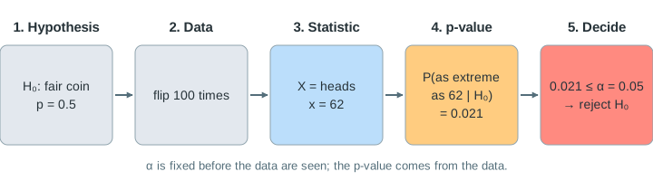
The canvas shows the recipe on one coin. The top chart is what H₀ predicts, the bottom chart is the coin as it really is (you choose it; the test never sees it), and the table on the right counts the four ways a decision can turn out.
Null and alternative hypotheses
The null hypothesis H₀ is the claim of "no effect" that the test tries to knock down: here p = 0.5, the coin is fair. The alternative H₁ is what we accept if H₀ falls: p ≠ 0.5. This H₁ is two-sided: too many heads and too few tails both count as evidence. A test never proves H₀; it only finds the data consistent or inconsistent with it.
The test statistic and its null distribution
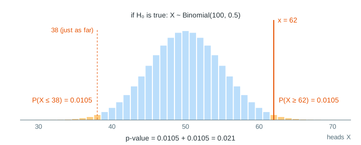
The 100 flips are squeezed into one number, the test statistic: X = the number of heads. If H₀ is true, X follows the binomial distribution Binomial(100, 0.5): mean 50, standard deviation 5. That is the top chart, the null distribution. Each bar is P(X = k) = C(100, k) / 2100 (see Pascal's triangle for where C(n, k) comes from).
The p-value is a tail area
The p-value is the probability, if H₀ is true, of a result at least as extreme as the one observed. For 62 heads, "at least as extreme" means at least 12 away from 50, on either side:
p = P(X ≥ 62 or X ≤ 38 | p = 0.5) = 0.0105 + 0.0105 = 0.0210On the canvas this is the orange area: the bars in both tails beyond the observed x (Demo: 62 heads → p = 0.021, reject H₀). 60 heads looks almost as odd, but its tails hold p = 0.0569 (Demo: 60 heads → p = 0.057, keep H₀).
| heads x | distance from 50 | two-sided p-value | at α = 0.05 |
|---|---|---|---|
| 58 | 8 | 0.1332 | keep H₀ |
| 60 | 10 | 0.0569 | keep H₀ |
| 61 | 11 | 0.0352 | reject H₀ |
| 62 | 12 | 0.0210 | reject H₀ |
| 65 | 15 | 0.0035 | reject H₀ |
α and the rejection region
The significance level α is chosen before looking at the data: how small a p-value must be to reject H₀. Rejecting when p ≤ α is the same as rejecting when X lands in the rejection region: the most extreme outcomes whose total probability under H₀ is at most α (the red bars). X can only be a whole number, so the region cannot hit α exactly; its real size is a bit less (Demo: α sets the rejection region).
| α | reject H₀ when | real size | power if p = 0.6 | power if p = 0.65 |
|---|---|---|---|---|
| 0.10 | X ≤ 41 or X ≥ 59 | 0.0886 | 62.3% | 91.2% |
| 0.05 | X ≤ 39 or X ≥ 61 | 0.0352 | 46.2% | 82.8% |
| 0.01 | X ≤ 36 or X ≥ 64 | 0.0066 | 23.9% | 62.7% |
Type I and type II errors
The test sees only X; the truth about the coin is hidden. So there are four outcomes:
| keep H₀ | reject H₀ | |
|---|---|---|
| H₀ true (fair coin) | correct, 1 − α | type I error (false alarm), α |
| H₀ false (biased coin) | type II error (missed effect), β | correct, power = 1 − β |
With a fair coin, every rejection is a false alarm, and α caps how often that happens. Repeating the test 100 times on a fair coin rejects 3 times, close to the real size 3.5% (Demo: type I errors with a fair coin). Medical screening has the same table: a false positive is a type I error, a missed disease a type II error (see Bayes' theorem for why a "significant" positive can still be more likely false than true).
Power
The power of a test is the chance it rejects H₀ when H₀ is false. It is not one number: it depends on how far the truth is from H₀. On the bottom chart, power is the green area of the real coin's distribution inside the red region, and β is the rest. A 60% coin is caught only 46% of the time with 100 flips at α = 0.05: 48 of 100 repeated tests in Demo: power against a 60% coin; a 65% coin, 83% of the time.
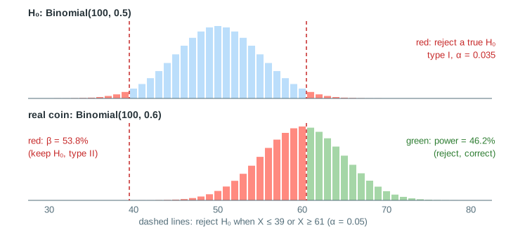
Three things raise power: a bigger true effect, more data (with n = 400 flips a 60% coin is caught almost always, because the spread of X/n shrinks like 1/√n, see the central limit theorem), and a larger α. The last one costs more false alarms: shrinking α from 0.05 to 0.01 cuts the power against a 60% coin from 46% to 24% (Demo: smaller α, less power). Studies choose n in advance so that power is at least 80% for the smallest effect worth finding.
What a p-value is not
- It is not the probability that H₀ is true. It is computed assuming H₀ is true.
- p > α does not show the coin is fair; the test may simply lack power (60 heads keeps H₀ although a 60% coin produces it often).
- A tiny p-value does not mean a big effect: with a million flips, 50.2% heads is "significant".
- Running many tests and reporting the one with p ≤ 0.05 makes false alarms almost certain (p-hacking).
For a normal statistic the same logic uses z-scores and the bell curve instead of binomial bars, see normal distribution, z-scores and confidence intervals; a 95% confidence interval excludes a value exactly when the two-sided test of that value rejects at α = 0.05.
What the page leaves out
- One-sided tests (H₁: p > 0.5), which put all of α in one tail.
- The normal approximation z = (X − 50)/5 and the continuity correction; the page uses exact binomial probabilities.
- Other tests: t-tests, chi-square, permutation tests, tests comparing two groups (A/B tests).
- Multiple-testing corrections (Bonferroni, false discovery rate) and sequential tests that peek as data arrives.
- Bayesian alternatives: Bayes factors and posterior probabilities for p itself.