The idea: add up many small random things and you get a bell
Roll one die and every face from 1 to 6 is equally likely: a flat histogram. Roll two and add them, and 7 is the most common sum while 2 and 12 are rare: a triangle. Roll five and add them, and the histogram of the sum is already a smooth bell. The central limit theorem (CLT) says this always happens: the sum of many independent random values with the same distribution is close to a normal distribution, whatever the shape of one value was.
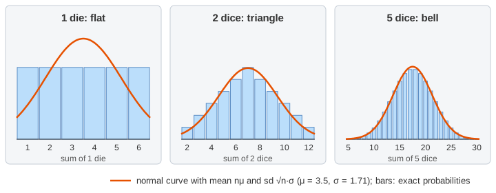
The page rolls n dice at a time with a seeded random generator, adds the faces and drops the sum into a histogram. The orange curve is the normal curve the theorem predicts, scaled to the number of rolls N. Demo: 1 die, flat and Demo: 2 dice, triangle start with one slow roll so you can follow a sum from the dice to its bar.
The mean and sd of a sum
One fair die has mean μ = 3.5 and standard deviation σ = √(35/12) ≈ 1.71. For a sum of n independent dice:
- the means add: mean of the sum =
nμ; - the variances add, not the sds: variance =
nσ², so sd =√n·σ.
The theorem adds the shape: for large n, (sum − nμ) / (√n·σ) is close to a standard normal
variable. The page draws exactly that curve, N(nμ, nσ²), over the bars.
| Dice n | Sums | Mean nμ | sd √n·σ | Shape |
|---|---|---|---|---|
| 1 | 1–6 | 3.5 | 1.71 | flat |
| 2 | 2–12 | 7 | 2.42 | triangle |
| 5 | 5–30 | 17.5 | 3.82 | bell |
| 16 | 16–96 | 56 | 6.83 | bell, narrow next to its range |
The range of the sum grows like n, but its sd only like √n. That is why the bell for 16 dice uses only the middle part of the 16–96 axis (Demo: 5 dice, bell curve).
Why two dice make a triangle
Two dice have 6 × 6 = 36 equally likely face pairs. Only (1,1) gives 2, but six pairs give 7: (1,6), (2,5), (3,4), (4,3), (5,2), (6,1). The counts 1, 2, 3, 4, 5, 6, 5, 4, 3, 2, 1 make the triangle. With more dice the number of ways to reach each sum keeps piling up in the middle, the same way the numbers in the middle of Pascal's triangle grow: the binomial coefficients are the "dice" with two faces, 0 and 1, and their rows turn into a bell too.
Any source, as long as σ is finite
The theorem does not need a fair die. The loaded die on the page lands on 1 with probability 0.40 and on 6 with only 0.04 (μ = 2.29, σ = 1.43): a steep, skewed shape. One loaded die gives a skewed histogram, 3 loaded dice are still lopsided with a long right tail, and the sum of 10 is close to the bell (Demo: loaded die still turns normal).
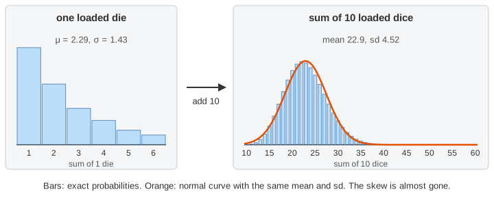
Two things the theorem does need: the values must be independent (or only weakly dependent), and one value must have a finite variance. A heavy-tailed source like the Cauchy distribution has no finite σ, and its averages never settle into a bell.
The sample mean gets steadier like 1/√n
Divide the sum by n and you get the sample mean x̄. Its mean is μ and its sd, the
standard error, is √n·σ / n = σ/√n. The panel on the right of the canvas measures
sd(x̄) for each n you have rolled and draws σ/√n as a bar. With σ = 1.71: 1 die gives 1.71, 4 dice 0.85,
16 dice 0.43 (Demo: spread of the mean, 1/√n).
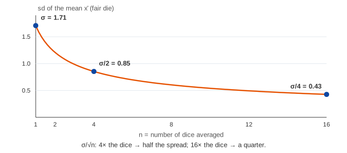
This is the rule behind every error bar and every Monte Carlo estimate: to make an average twice as precise you need four times the data. Monte Carlo estimation of π shows the same 1/√n error with random points in a square.
The sum or mean that turns normal here is put to work in the Normal Distribution page: z-scores, percentiles and 95% confidence intervals.
See also Mean vs Median vs Mode, which shows how far one outlier drags the mean compared with the median.
When p is small instead of n·p large, the binomial count goes Poisson, not normal: see Binomial vs Poisson.
The Confidence Intervals page uses that standard error to build x̄ ± 1.96·σ/√n and shows about 95% of them catching μ.
What the page leaves out
- The formal statement (Lindeberg–Lévy) and its proof with characteristic functions.
- How fast the bell appears: the Berry–Esseen bound says the error shrinks like 1/√n and grows with the skew of the source.
- Versions for values that are not identically distributed (Lyapunov, Lindeberg) or weakly dependent.
- The continuity correction: the page compares a discrete sum with a continuous curve directly.
- The law of large numbers, which only says x̄ → μ; the CLT also gives the shape and size of the error.