The idea: try the machines, or play the best one so far?
A multi-armed bandit is a row of slot machines (arms). Each pull of an arm pays 1 or 0, and each arm pays 1 with its own chance p that the player does not know. The player has a fixed number of pulls and wants as much total reward as possible.
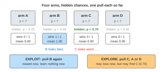
Every pull is a choice between two goals. Exploit: pull the arm that looks best so far, to collect reward now. Explore: pull an arm that is less known, to learn whether it is better. Too little exploring can lock the player onto a worse arm; too much wastes pulls on arms already known to be bad. This is the explore–exploit trade-off, and the bandit is its simplest form: no states, just arms and rewards.
The page has four arms with p = 0.25, 0.50, 0.70 and 0.40, so C is the best. A run is 300 pulls. Pick a strategy and press Pull Once to see one choice in detail, or Run 300 Pulls for a whole run. Every strategy sees the same luck: the 5th pull of C wins or loses the same way in every run, so the runs differ only in their choices.
Regret
A strategy is measured by its regret: how much reward it lost against a player who knew the answer and always pulled C. Each pull of arm i adds 0.70 − pi, so a pull of B costs 0.20, a pull of A 0.45, and a pull of C nothing. The chart under the arms draws the cumulative regret of each run as it goes.
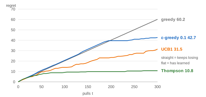
A strategy that never stops making mistakes has regret that grows in a straight line. A good strategy makes fewer and fewer mistakes, so its curve bends and flattens. The best possible regret grows like log T (Lai and Robbins, 1985): you can never be sure, so a little exploring never stops, but it can become very rare.
Greedy and ε-greedy
Greedy pulls each arm once, then always pulls the arm with the highest mean wins / pulls. On the page, C's first pull loses and B's first pull wins, so greedy sees B at 1.00 and C at 0.00. From then on it pulls only B. B's mean settles near 0.50 but never drops to 0, so C is never tried again and regret grows by 0.20 per pull, to 60.2 (Demo 2).
ε-greedy does the same but, with probability ε, pulls a random arm instead. Random pulls eventually give C enough wins for its mean to pass B's, and then C is exploited. But the random pulls never stop: with ε = 0.1 about 1 pull in 10 is still random, a quarter of them on A, so regret keeps growing in a straight line, just a gentler one (Demo 3). Larger ε finds C sooner but pays more later; the value is in Options.
UCB1: optimism for what you know little about
UCB1 (upper confidence bound, Auer, Cesa-Bianchi and Fischer, 2002) gives each arm a score:
score(i) = mean(i) + √( 2 · ln t / n(i) )Here t is the number of pulls so far and n(i) the pulls of arm i. The second term is a bonus for uncertainty: it is large for an arm pulled few times and shrinks as the arm is pulled. Each pull of an arm shrinks its own bonus, while the slowly growing ln t lets the bonus of a neglected arm creep up until it is tried again. The idea is called optimism in the face of uncertainty: treat each arm as good as it could plausibly be.
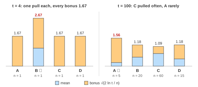
On the canvas the blue bar is the mean and the orange part on top is the bonus (Demo 1 steps through the first six pulls). In a full run UCB1 tries every arm a fair number of times and then settles on C; its regret bends (Demo 4). Its bonus is cautious, so in 300 pulls it still explores more than it needs to.
Thompson sampling
Thompson sampling (Thompson, 1933) keeps a belief about each arm's p: a Beta(1 + wins, 1 + losses) distribution, which starts flat (Beta(1, 1): any p is equally likely) and gets narrower with every pull. For each pull it draws one random value θ from each arm's belief and pulls the arm with the highest θ.
An arm that is clearly worse almost never draws the highest θ. An arm that is still uncertain sometimes draws high and gets tried. So each arm is pulled about as often as the chance that it is the best. On the canvas the purple bar is the likely range of the belief and the red mark is this pull's θ (Demo 5, Demo 6). On the page Thompson ends at regret 10.8, the lowest of the four (Demo 7).
| strategy | how it explores | regret after 300 pulls on the page |
|---|---|---|
| greedy | never (after one pull each) | 60.2, locked on B |
| ε-greedy, ε = 0.1 | at random, forever | 42.7, still growing linearly |
| UCB1 | bonus for few pulls, shrinking | 31.5, bending |
| Thompson sampling | random draws from Beta beliefs | 10.8, almost flat |
These numbers come from one luck table, so treat them as an example. Over many runs Thompson sampling and tuned UCB variants both reach the log T rate, and Thompson is often ahead in practice.
Where bandits are used
- A/B tests that adapt: send more traffic to the variant that is winning while the test runs, instead of a fixed 50/50 split (see A/B Testing).
- Ads, news and recommendations: each item is an arm; a click is a reward. With user features this becomes a contextual bandit (LinUCB).
- Game-tree search: Monte Carlo Tree Search picks which child to explore with UCT, which is UCB1 applied at each node.
- Reinforcement learning: a bandit is reinforcement learning with one state. With many states and delayed rewards the same trade-off shows up as ε-greedy in Q-Learning; Supervised vs Unsupervised vs Reinforcement Learning places it among the kinds of learning.
See also Bayes' Theorem for the belief update behind Thompson sampling, and Value Iteration for planning when the rewards are known.
With states and whole episodes instead of single pulls, the same idea of nudging action probabilities by reward becomes Policy Gradient: REINFORCE.
What the page leaves out
Many runs and average regret (the page shows one luck table); rewards that are not 0 or 1; arms whose chances change over time (non-stationary bandits and discounting); contextual bandits; adversarial bandits (EXP3); tuned UCB variants such as KL-UCB; pure exploration (best-arm identification); and the lower-bound proof.