Matrix Factorization Visualization | Recommendations Learned by SGD

The idea: fill in the empty cells

A shop knows a few ratings: Ann gave Alien 5 and Titanic 1, Fay rated only Titanic. Most cells of the ratings matrix R (users × films) are empty. A recommender has to guess the empty cells and show each user the films with the highest guesses. Guessing from what similar users liked is called collaborative filtering.

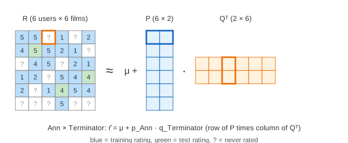
A 6 by 6 ratings matrix with known ratings and question marks is approximately the mean mu plus a 6 by 2 user matrix P times a 2 by 6 film matrix Q transposed. Each cell is the dot product of a user's row of P and a film's column of Q transposed — 36 cells are explained by 24 numbers: one 2-number vector per user and one per film. The empty cells come for free.

Matrix factorization gives every user u a short vector p_u and every film i a vector q_i, here with k = 2 numbers each (the latent factors). The predicted rating is

r̂(u, i) = μ + p_u · q_i = μ + p_u1 q_i1 + p_u2 q_i2

where μ = 3.14 is the mean of the 21 training ratings. Stack the user vectors into a 6 × 2 matrix P and the film vectors into a 6 × 2 matrix Q, and all predictions together are μ + P Qᵀ: a 6 × 6 matrix built from two thin ones. That is why it is called a factorization. On the canvas, P sits left of the ratings and Qᵀ above them, so each cell lines up with its row of P and its column of Qᵀ.

Three ratings (green cells) are kept back as a test set. Training never sees them; they show how well the model guesses ratings it has not seen.

Predict, error, update

The vectors start as small random numbers, so every prediction is close to μ. Training wants a small squared error on the known ratings, plus a penalty on large vectors:

minimize  Σ over known (u, i):  (r − μ − p_u · q_i)²  +  λ (|p_u|² + |q_i|²)

Stochastic gradient descent (SGD) takes one known rating at a time (Demo 1):

Predict r̂ = μ + p_u · q_i.
Error e = r − r̂. Positive means the guess was too low.
Update both vectors, using the old values on the right:
p_u ← p_u + η (e · q_i − λ · p_u)
q_i ← q_i + η (e · p_u − λ · q_i)

The update is the gradient of the squared error (the factor 2 is folded into η). When e > 0 the user vector moves toward the film vector and the film vector toward the user vector, so their dot product grows; when e < 0 they move apart. The λ term pulls both a little toward 0. One pass over all 21 training ratings is an epoch (Demo 2); the page visits them row by row. See Gradient Descent for the learning rate in general.

The latent space

Each p_u and q_i has two numbers, so they can be drawn as points in a plane. The dot product p · q is large when the two points lie in the same direction from the origin and far from it, and negative when they point opposite ways. After 40 epochs (Demo 3) Ann, Bob and Cat sit with Alien, Matrix and Terminator on one side of the f2 axis, and Dan, Eve and Fay with Titanic, Notebook and Amélie on the other.

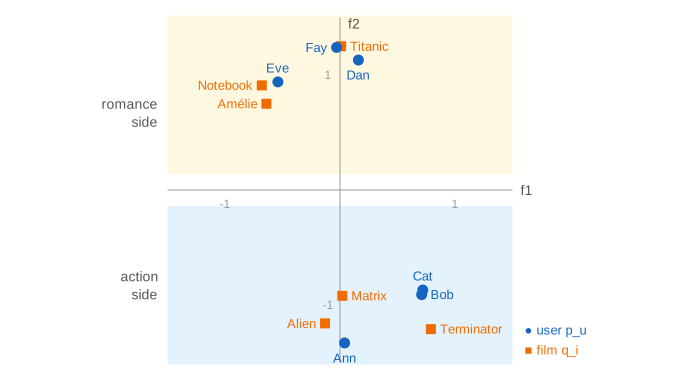
Latent space after 40 epochs with eta 0.1 and lambda 0.3. Users Ann, Bob, Cat and films Alien, Matrix, Terminator have negative f2, near minus 1. Users Dan, Eve, Fay and films Titanic, Notebook, Amélie have positive f2, near plus 1 — Nobody told the model about genres: the second factor became "action versus romance" because that explains the ratings best.

The model was never told which films are action films. It found an axis that explains the ratings, and that axis happens to be the genre. This is the core idea of learned embeddings: useful coordinates for things, learned from how they are used. The axes have no fixed meaning, though: another random start can give the same picture rotated or mirrored, with the same predictions. The first factor here carries little, because two groups need only one direction.

To recommend, predict every ? cell of the user's row and take the highest. Ann has not rated Terminator or Notebook; the model predicts 4.8 and 1.9, so it recommends Terminator (Demo 3). A pick below 3.5 is shown grey: nothing left is worth recommending.

Fay rated only Titanic, 5. That one rating is enough to pull her vector toward Titanic's, into the romance group, so her top pick is Notebook, 4.3 (Demo 4). A user with no ratings at all would keep her small random start vector and get μ for every film: the cold start problem. Real systems fill that gap with popular items, a short sign-up quiz, or features of the user and the item.

Regularization and the learning rate

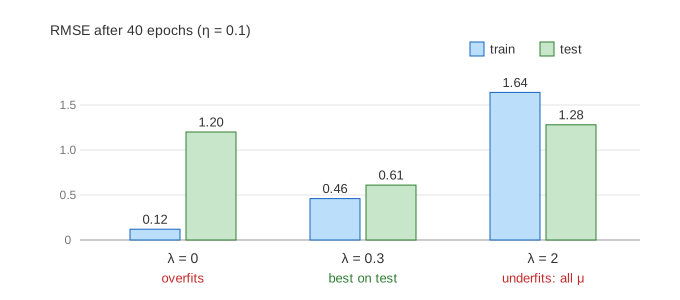
Here 21 ratings are fitted with 24 numbers, so the model can fit them almost exactly and still guess badly elsewhere. That is overfitting, and λ fights it by keeping vectors short.

Train and test RMSE after 40 epochs for three values of lambda. Lambda 0: train 0.12, test 1.20, overfits. Lambda 0.3: train 0.46, test 0.61, best test error. Lambda 2: train 1.64, test 1.28, every prediction is the mean, underfits — Lowest training error is not the goal: λ = 0 fits the training ratings best and the test ratings worst.

setting (40 epochs)	train RMSE	test RMSE	what happens
η = 0.1, λ = 0.3	0.46	0.61	good fit, genres separate (Demo 3)
η = 0.1, λ = 0	0.12	1.20	overfits: test error rises after epoch 10 (Demo 5)
η = 0.1, λ = 2	1.64	1.28	underfits: all vectors shrink to 0, every cell is μ (Demo 6)
η = 0.01, λ = 0.3	1.11	1.00	too slow: still learning after 40 epochs
η = 0.8, λ = 0.3	—	—	diverges in epoch 2 (Demo 7)

With a learning rate that is too big, each step overshoots: the error after the step is bigger than before, the next step is bigger still, and the vectors blow up. With one that is too small, the model needs many more epochs. In practice λ and η are chosen by trying a few values and keeping the ones with the lowest error on held-out ratings.

In practice

Netflix Prize (2006–2009): Simon Funk's SGD factorization (often called "Funk SVD") and its extensions with user and item biases were the core of the winning blends.
Alternating least squares (ALS): fix Q and solve for every p_u exactly (a small least-squares problem, see Linear Regression), then fix P and solve for Q, and repeat. Easy to run in parallel, as in Spark MLlib.
Implicit feedback: clicks, plays and purchases instead of stars; every missing cell counts as a weak "no" with a low confidence weight.
Not the same as SVD: a plain SVD needs every cell filled in. Matrix factorization fits only the known cells, which is what makes it work on a mostly empty matrix.

See also K-Means Clustering for grouping points without labels, and Retrieval-Augmented Generation and HNSW Vector Search for finding the nearest vectors among millions.

What the page leaves out

User and item biases (b_u, b_i: Cat rates everything high); shuffling the ratings each epoch; more factors than two; ALS and other solvers; implicit feedback and weighted losses; ranking metrics such as precision@k; time effects; and the scale of real systems with millions of users, sparse storage and negative sampling.