The idea: a graph you can walk to the nearest vector
A vector database stores embeddings: lists of numbers where similar things get nearby points.
The question it answers all day is k-nearest neighbours: which k stored vectors are closest to this query vector?
Comparing the query with every vector is exact but costs N distance computations per query.
HNSW (Hierarchical Navigable Small World) builds a graph instead: each vector is linked to a few near vectors,
and a search walks along the links towards the query. It is the default index in pgvector, Qdrant, Weaviate, Milvus,
Elasticsearch and FAISS (IndexHNSWFlat).
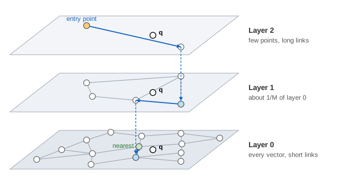
The canvas shows 40 vectors in two dimensions (real embeddings have hundreds), drawn once per layer: layer 2 on the left,
layer 1 in the middle, layer 0 on the right. Press Search to find the 3 nearest vectors to q, change
ef, press Brute force to get the exact answer, or Insert vector to add one.
Click layer 0 to move q.
Layers and random levels: the skip-list idea
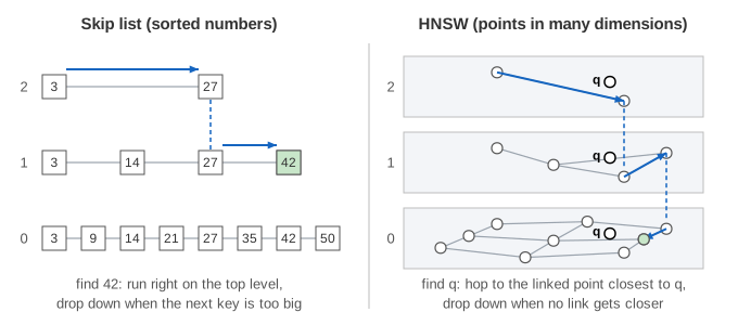
Every vector is in layer 0. When a vector is inserted it draws a random level ℓ = ⌊−ln(u) · mL⌋ with u uniform in (0, 1] and mL = 1/ln(M), and it is stored in layers 0 to ℓ. So each layer holds about 1/M of the layer below. With M = 3 here, about a third of the vectors reach layer 1 and a ninth layer 2 (the seeded data gives 40, 13 and 3). This is the same trick as a skip list: a few express lanes on top, every element on the bottom, and a search that starts high and drops down.
Search: greedy on top, beam search on layer 0
- Start at the entry point on the top layer (the “ep” tag on the canvas).
- On each upper layer, walk greedily: look at the linked points, move to the one closest to q, and stop when none is closer. That point is the entry point for the layer below.
- On layer 0, run a beam search. It keeps a candidate list C (points to explore, nearest first) and a result list
W (the best
efpoints so far). Take the nearest candidate, compute the distance to each of its unseen links, and put a point into C and W if W is not full or it beats the worst result in W. Stop when the nearest candidate is farther than the worst result. - Return the k best points of W.
The canvas colours a point blue when its distance has been computed, orange while it is in W, green when it is returned and truly among the 3 nearest, and red when it is one of the true 3 nearest but the search missed it. (Demo: one search, step by step.)
ef: speed against recall
HNSW is approximate. The greedy walk and the beam can stop in a pocket of the graph that is near q but not
the nearest. Recall@k is the fraction of the true k nearest that the search returns. A bigger
ef keeps more results, explores more candidates, computes more distances and finds the true neighbours more often.
(Demo: recall vs ef: for q = (25, 10), ef = 3 returns 2 of the true 3 after 12 distance computations; ef = 12 returns all 3 after 26.)
| Setting | Bigger value gives | Costs |
|---|---|---|
ef (query time; ef_search in pgvector) | higher recall | more distance computations per query |
M (links per insert) | better connected graph, higher recall | more memory, slower inserts and searches |
ef_construction | better links chosen at insert | slower index build |
Insert: draw a level, search, link to M nearest
Inserting a vector is mostly a search for it. Draw its level ℓ. Walk greedily from the entry point down to layer ℓ.
Then on each layer from ℓ down to 0, run the beam search with ef_construction (8 here), link the new vector to its
M nearest finds (3 here), and add the links back. A point whose list now has more than
Mmax links (3 on upper layers, Mmax0 = 2M = 6 on layer 0) keeps only its nearest. Links in hnswlib are
one-way lists, so a dropped link can still exist in the other direction; the canvas draws a line while either direction exists.
If the new vector's level is above the top layer, it becomes the new entry point. (Demo: insert a vector.)
HNSW vs brute force
Brute force (a flat index) computes the distance from q to every vector: exact, simple, and O(N) per query. HNSW looks at a small, slowly growing part of the vectors: about O(log N) hops, each looking at up to M links. With only 40 vectors the saving on the canvas is about 2× (Demo: HNSW vs brute force); it grows with N.
| Vectors N | Brute force distances | HNSW distances (typical) |
|---|---|---|
| 40 (this page) | 40 | about 12–30 |
| 1 million | 1,000,000 | a few thousand |
| 1 billion | 1,000,000,000 | tens of thousands (if the graph fits in memory) |
The price: the graph uses extra memory (M to 2M links per vector), inserts are slower than appending to a list, deletes are hard (most systems mark a vector deleted and clean up later), and recall is not guaranteed.
Where it is used
In retrieval-augmented generation the question is embedded and the vector index returns the top_k chunks: that lookup is usually an HNSW search. The same index serves recommendations, image search and de-duplication. K-nearest neighbours classification needs the same query; k-means is the idea behind the other popular index family (IVF: cluster the vectors, search only the nearest clusters). Embeddings themselves come out of models like the ones on the attention and LLM pages.
HNSW layers work like the express lanes of a skip list.
HNSW finds the nearest vectors fast, but nearest is not always relevant: BM25 vs Vector Search vs Hybrid shows where dense search misses exact codes and how hybrid search with RRF fixes it.
What the page leaves out
Real embeddings have 384–3072 dimensions and use cosine or dot-product distance; the page uses 2-D points and Euclidean distance so the graph can be drawn. Levels are capped at 2, and the parameters are tiny (M = 3; real defaults are M = 16, ef_construction = 64–200). The neighbour choice is the simple “M nearest” rule, not the paper's heuristic that prefers links in different directions. Not shown: deletes, filtered search, quantization (PQ, scalar), on-disk variants such as DiskANN, concurrency, and how the index is persisted.