The idea: a cluster is a dense region
DBSCAN (Density-Based Spatial Clustering of Applications with Noise) does not look for centres. It looks for places where points are packed closely, and joins packed places that touch into one cluster. Points in empty space belong to no cluster: they are noise. You do not choose the number of clusters, and a cluster can have any shape.
Two parameters: eps and minPts
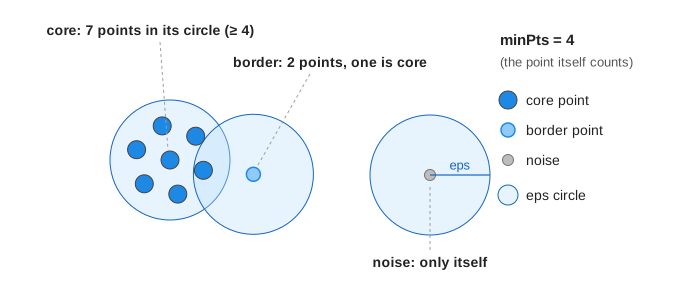
eps (ε) is a radius: the eps-neighbourhood of a point is every point
within distance eps of it, the point itself included. minPts is how many points a
neighbourhood needs to count as dense (scikit-learn calls it min_samples, default 5).
On the canvas the shaded disc is the eps-neighbourhood of the point being looked at, and the grey lines go
to its neighbours.
| Kind | Rule | On the canvas |
|---|---|---|
| core | at least minPts points within eps | big dot in the cluster colour |
| border | fewer than minPts, but within eps of a core point | smaller, lighter dot |
| noise | fewer than minPts and no core point within eps | small grey dot |
A common starting point is minPts = 2 × the number of dimensions (4 for the page's 2-D data).
Growing a cluster: a queue of density-reachable points
The scan visits the points in number order. A point that is not yet labelled gets its neighbourhood counted:
- Fewer than minPts: mark it noise for now and go on.
- At least minPts: it is core, a new cluster starts, and all its neighbours go into a queue (yellow on the canvas).
- Take the next point from the queue and put it in the cluster. If it is core too, its own unlabelled neighbours join the queue. If not, it is a border point and adds nobody. A point that was marked noise earlier becomes a border point here.
- When the queue is empty, the cluster is complete. The scan goes on.
A point that can be reached through a chain of core points, each within eps of the next, is density-reachable. The queue is exactly a breadth-first search over the graph "core point → every point within eps", so a cluster is a connected component of that graph, with border points hanging off its edge. (Demo 1: two moons: the scan marks the outlier #1 and the moon tip #2 as noise (only 3 points within eps), #3 starts cluster 1, the queue walks along the whole upper moon, and #2 is claimed back as a border point.)
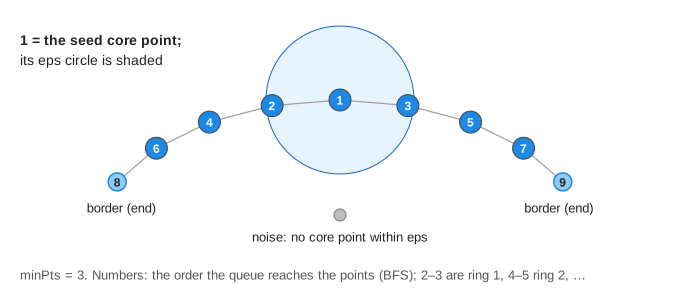
With the blobs data and eps = 1.0, minPts = 4 the run ends with 3 clusters: 33 core, 3 border and 6 noise points (the 4 planted outliers and 2 stragglers of the sparse blob). (Demo 2: core, border and noise)
Why K-Means fails on moons and rings
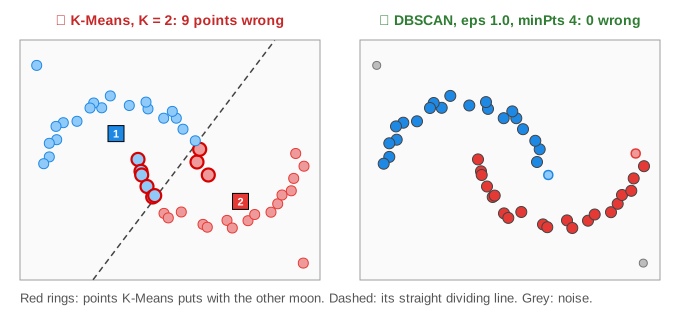
K-Means gives every point to its nearest centre. Between two centres the dividing line is straight, so each cluster is a convex blob around its centre. Two half-moons that hook into each other cannot be cut apart by a straight line, and a ring has no compact centre at all.
| Data | K-Means (K = true number) | DBSCAN (eps 1.0, minPts 4) |
|---|---|---|
| two moons, 46 points | 9 points in the wrong moon | 2 clusters, 0 wrong, 2 outliers are noise |
| two rings, 55 points | 27 points wrong: both rings cut in half | 2 clusters, 0 wrong, 1 outlier is noise |
| three blobs, 42 points | 0 wrong, but the 4 outliers forced into clusters | 3 clusters, the outliers are noise |
(Demo 3 and Demo 4 run K-Means first, outline its mistakes in red, then run DBSCAN on the same points.)
Choosing eps: too small, too big
- Too small (eps = 0.3): no point has 4 points that close, so nothing is core and all 46 points are noise. (Demo 5)
- Too big (eps = 2.0): the gap between the moons (1.54 at its narrowest) is smaller than eps, a chain of core points crosses it, and both moons become one cluster. (Demo 6)
- minPts too high (8 on the blobs): the sparse blob never has 8 points within eps, so its 12 points turn to noise and only 2 clusters are left. (Demo 7)
A standard way to pick eps is the k-distance plot: for every point, compute the distance to its k-th nearest neighbour (k = minPts − 1), sort these distances and plot them. Points inside clusters have small values, noise has large ones; choose eps at the "knee" where the curve turns sharply upward.
Cost and details
- Each point asks for its neighbourhood once. Done naively that is n distance computations per query, O(n²) in total; with a spatial index (k-d tree, ball tree, R-tree) it is about O(n log n) for low dimensions.
- Core points and noise do not depend on the scan order. A border point within eps of core points of two different clusters goes to whichever cluster reaches it first, so it can depend on the order.
- One eps for the whole space means DBSCAN struggles when clusters have very different densities; OPTICS and HDBSCAN handle that by looking at all eps values at once.
- Like any distance-based method (see k-nearest neighbours), features on different scales should be standardized first.
Joining overlapping neighbourhoods into clusters is the same job a union-find structure does: some DBSCAN implementations union every core point with its core neighbours instead of using a queue. For connected components in a directed graph, see strongly connected components.
See also PCA vs t-SNE, two ways to flatten data to 2-D, and why gaps between groups in a t-SNE plot are not distances.
What the page leaves out
The data is 2-D with at most 55 points, and every neighbourhood is found by checking all points; real implementations use a spatial index and work in many dimensions, where distances become less meaningful. The page does not draw the k-distance plot, and only describes OPTICS, HDBSCAN and the order dependence of border points. Distances are Euclidean; other metrics (Manhattan, cosine, haversine for map points) work the same way.