The idea: how far from the mean, on average?
The mean tells you where the data sits. The next question is how spread out it is: are the scores bunched near the mean, or scattered far from it? The variance answers with one number: the average of the squared distances from the mean. The standard deviation is its square root, so it is back in the data's own units.
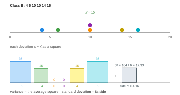
The page takes six quiz scores and works the recipe one step at a time. Each score keeps one colour from its dot on the dot plot to its deviation bar, its table row and its square (Demo: tight class, step by step).
Why square the deviations?
A deviation is x − x̄: how far one score is from the mean, with a sign. Scores
below the mean give negative deviations, scores above give positive ones. Because the mean is the balance
point, they always add up to exactly 0. Their plain average is 0 for every data set, so it says nothing about
spread.
Squaring removes the sign: (−4)² = 16 and 4² = 16. It also weighs far scores more:
twice as far gives four times the area. Another fix is to take absolute values, which gives the
mean absolute deviation. Squares are used far more often because they have neater algebra,
and the normal distribution is built on them.
The formulas
| Quantity | Formula | Class B (4 6 10 10 14 16) |
|---|---|---|
| mean | x̄ = Σx / n | 60 / 6 = 10 |
| sum of squares | Σ(x − x̄)² | 36 + 16 + 0 + 0 + 16 + 36 = 104 |
| variance | σ² = Σ(x − x̄)² / n | 104 / 6 = 17.33 points² |
| standard deviation | σ = √σ² | √17.33 = 4.16 points |
The variance is in squared units (points², cm², $²), which is hard to picture. The standard deviation is
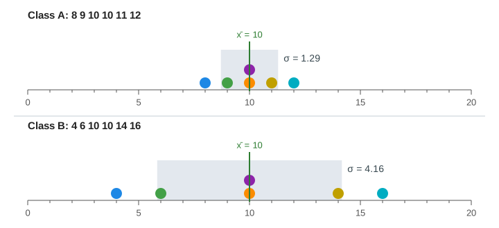
in the same units as the data, so you can draw it on the dot plot: the grey band x̄ ± σ shows
where a "typical" score lies.
Same mean, different spread
Class A scored 8 9 10 10 11 12 and Class B scored 4 6 10 10 14 16. Both have mean 10, so the mean alone cannot tell them apart. Class A's squares are tiny (Σ = 10, σ = 1.29); Class B's are big (Σ = 104, σ = 4.16). Demo: same mean, wider spread.
Outliers, shift and scale
- One outlier. Change Class A's 12 into 24 and the mean moves to 12. That one score is 12 points away, so its square has area 144 out of a total of 178. σ jumps from 1.29 to 5.45. Like the mean, σ is not robust (Demo: one outlier, one huge square).
- Shift. Add 5 to every score: the mean moves by 5, but every deviation stays the same, so the variance and σ do not change.
- Scale. Double every score: every deviation doubles, every square grows 4×, the variance
grows 4× and σ doubles (1.29 → 2.58). In general
sd(a + kx) = |k|·sd(x)(Demo: shift +5 and scale ×2).
Population n vs sample n − 1
If the six scores are the whole group you care about, divide by n: that is the population
variance σ². If they are a sample from a bigger group and you want to estimate that
group's spread, divide by n − 1 instead: the sample variance s². The sample mean
is fitted to the sample, so the sample's points sit a little closer to it than to the true mean. Dividing by
n would make the estimate too small on average; n − 1 (Bessel's correction) fixes that. For Class B,
s² = 104 / 5 = 20.80 and s = 4.56, versus σ = 4.16. The gap shrinks as n grows
(Demo: sample n − 1 vs population n). Spreadsheets have both: VAR.P/STDEV.P
and VAR.S/STDEV.S.
Where σ is used next
A z-score z = (x − μ)/σ measures distance from the mean in standard deviations, and in a bell
curve about 68% of values fall within one σ: see Normal Distribution.
The Central Limit Theorem page shows that variances (not standard
deviations) add when you sum independent values, and that the mean of n values has sd σ/√n. That standard
error is what Confidence Intervals are built from.
See also Mean vs Median vs Mode, which shows how far one outlier drags the mean compared with the median.
What the page leaves out
- Variance of a random variable,
Var(X) = E[(X − μ)²] = E[X²] − μ², and the shortcut formula for computing it from Σx and Σx². - Robust measures of spread: the interquartile range and the median absolute deviation.
- Why n − 1 makes s² unbiased (the proof), and why s itself is still slightly biased.
- Grouped data and weighted variance.
- Covariance and correlation, which measure how two variables spread together.
See where this page fits on the Probability & Statistics mind map.