The idea: every example says how it wants the network to change
A network learns by changing its 13,002 weights and biases so that its cost goes down. Backpropagation is how it finds out which way to change each one. This page shows the intuition from 3Blue1Brown's lesson on the same network as Neural Network: Recognizing Handwritten Digits (784 → 16 → 16 → 10, sigmoid), but starting from random weights and trained right in the page.
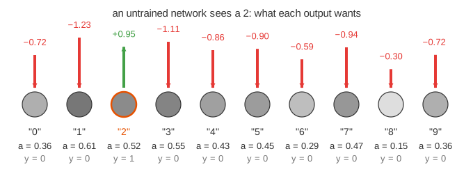
Take one training image, a 2. The cost of this one example is C = Σ (aj − yj)² over the 10 outputs, where y = 1 for output "2" and 0 for the others. With random weights the outputs are a mess: output "2" is 0.52, output "1" is 0.61, and the cost is 1.88. Each output wants to move toward its target, and how strongly is proportional to how far off it is: 2(y − a). Output "2" wants +0.95; output "1" wants −1.23, the most of any. (Demo 1)
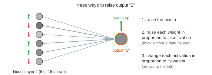
Three ways to raise an output
Output "2" computes a = σ(w·a(h2) + b) from the 16 activations of hidden layer 2. To make it bigger there are three knobs:
| knob | wanted change is proportional to | in words |
|---|---|---|
| its bias b | its own wish (times the sigmoid's slope) | lift the sum regardless of the input |
| its weights wk | the activation ak each weight carries | weights from active neurons matter most: "neurons that fire together wire together" |
| the activations ak of hidden layer 2 | the weight wk | up where w > 0, down where w < 0 |
The first two the network can do directly. The third it cannot: the activations of hidden layer 2 come from that layer's own weights and biases. So the third way becomes a wish passed to the layer before. (Demo 2)
Adding up the wishes, going backwards
Hidden layer 2 does not only feed output "2". All 10 outputs have a wish for it, and they disagree: "2" wants some neurons up, "1" wants them down. The wishes of all 10 outputs are added up, each through its weight (and the sigmoid's slope). The sum is what hidden layer 2 wants. Now repeat: hidden layer 2's wishes, through its weights, give hidden layer 1's wishes. Moving backwards layer by layer like this is backpropagation. It stops at the pixels: the image is data, not something to change.
The same wishes also give every weight's change: (the wish of the neuron it feeds) × (the sigmoid's slope there) × (the activation it carries). For a first-layer neuron the activations are the pixels, so its 784 weight changes form a picture of the 2 itself, blue or red depending on whether the neuron should turn up or down. (Demo 3) The exact formulas, with the chain rule, are on Backpropagation; this page computes exactly them (checked against finite differences).
Averaging over examples is the gradient
One 2 wants one set of changes; a 7 wants another. What actually helps the network is the change that most of the examples agree on. Run backpropagation on every training example and average the wishes: the result is the negative gradient of the total cost, the direction in the space of all 13,002 numbers that lowers the cost fastest. Taking a small step that way is gradient descent.
Stochastic gradient descent
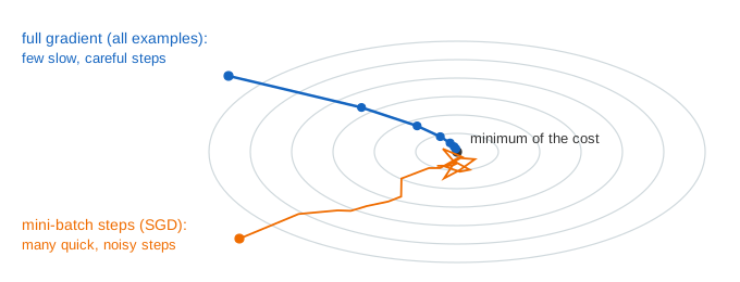
Averaging over all examples before every step is slow. Instead, shuffle the data, cut it into mini-batches (here 10 images; the lesson suggests about 100 out of MNIST's 60,000), average over one mini-batch and step right away. Each step is only a rough guess of the true downhill direction, so the path wobbles: a drunk man stumbling quickly downhill rather than a careful one taking slow, exact steps. But there are many more steps, and it gets down sooner. This is stochastic gradient descent. One pass through all the data is an epoch; after each epoch the page reshuffles the 100 images, so every epoch has different mini-batches. (Demo 4)
On this page: one mini-batch step takes the cost on all 100 training images from 2.09 to 0.93. The first epoch (10 steps) mostly teaches the network to say "no" to everything: all outputs drop near 0, which is already much cheaper than random outputs, but only 10 of 100 images are classified correctly. The real progress comes later: after 20 epochs (200 steps) the cost is 0.28, 87 of 100 are right, and output "2" on our 2 is 0.71. Its wishes have become small. (Demos 5–6)
| epochs | mini-batches of 10: cost (all 100) | correct | full gradient: cost | correct |
|---|---|---|---|---|
| 0 (random) | 2.09 | 10 / 100 | 2.09 | 10 / 100 |
| 1 | 0.92 (10 steps) | 10 / 100 | 0.92 (1 step) | 10 / 100 |
| 10 | 0.84 (100 steps) | 19 / 100 | 0.90 (10 steps) | 18 / 100 |
| 20 | 0.28 (200 steps) | 87 / 100 | 0.90 (20 steps) | 32 / 100 |
| 40 | 0.02 (400 steps) | 100 / 100 | 0.89 (40 steps) | 36 / 100 |
Both columns use every image the same number of times. The full gradient takes one exact step per epoch and is still stuck on the "say no to everything" plateau after 40 epochs; mini-batches take ten rough steps per epoch and get through it. That is why real training uses mini-batches. Switch between them with the batch select; after Reset the previous run stays on the cost curve in orange, so two runs can be compared. (Demo 7: full gradient vs mini-batches)
What the page leaves out
The calculus (the chain rule written out) is on Backpropagation. The data are 100 synthetic stroke digits, not MNIST's 60,000 handwritten ones; the shuffles come from a seeded random generator, so every run of the page gives the same numbers. The learning rate is fixed at η = 3 for both batch sizes. The cost is the lesson's squared error; real classifiers use softmax with cross-entropy, and optimizers such as momentum or Adam instead of plain SGD. Accuracy is measured on the training images themselves, not on new ones.