The idea: the wait between random arrivals
Buses come at random, on average λ per minute, each one independent of the others. This is a Poisson process. The time T you wait from one bus to the next is random too, and it follows the exponential distribution: short waits are the most common, long waits are rare but possible.
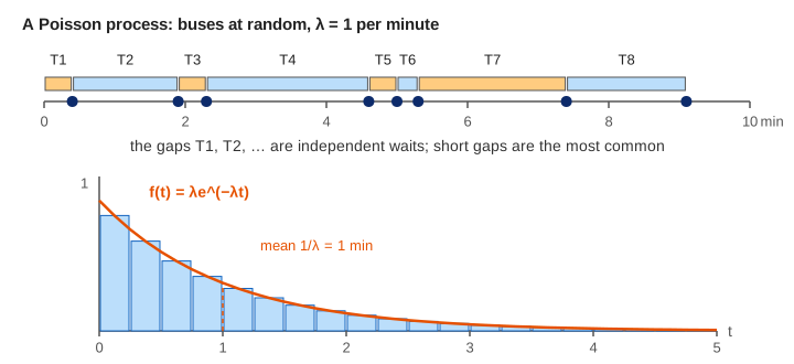
The canvas draws one 20-minute timeline, drops each gap into a histogram of waiting times and draws the curve λe−λt over it. The table compares the share of waits longer than t with e−λt. Demo: one 20-minute timeline follows the gaps from the timeline into the chart.
Density, survival and mean
For a rate λ per minute:
density      f(t) = λ · e^(−λt),   t ≥ 0
survival     P(T > t) = e^(−λt)
mean 1/λ     median ln 2 / λ     variance 1/λ²
The survival line comes straight from the Poisson count: no bus in the next t minutes means a Poisson(λt) count of 0, which has probability e−λt. With λ = 1:
| t (min) | 0.5 | 1 | 2 | 3 | 4 |
|---|---|---|---|---|---|
| P(T > t) = e−t | 0.6065 | 0.3679 | 0.1353 | 0.0498 | 0.0183 |
After 1000 seeded waits the observed shares sit within about 0.02 of these numbers and the observed mean is close to 1 (Demo: 1000 waits trace λe^(−λt)). The mean is larger than the median 0.69: a few long waits pull it up.
Changing the rate
Twice as many buses halves every wait. At λ = 2 the curve starts at height 2 and the mean wait is 0.5 min (Demo: faster buses, λ = 2); at λ = 0.5 it starts at 0.5, the mean is 2 min and the tail reaches past 8 minutes (Demo: slow buses, λ = 0.5, long tail). The y axis is scaled to 1.5λ, so the curve has the same shape on screen; only the numbers on the axes change. The first bar sits a little under the curve's start because it averages the density over its whole bin, 0 to 0.25 min.
Memoryless: the wait starts over
You have already waited s minutes. Is the bus now closer? For the exponential distribution, no:
P(T > s + t | T > s) = e^(−λ(s+t)) / e^(−λs) = e^(−λt) = P(T > t)This is the memoryless property. Demo: memoryless, already waited 2 min draws 10000 waits, throws away the ones that ended before s = 2 (about e−2 = 13.5% survive), and plots the remaining wait T − s of the rest. The purple histogram lies on the same curve λe−λt and its mean is still about 1/λ.
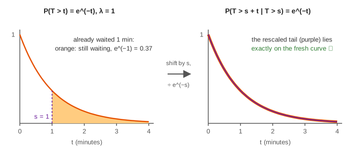
The exponential is the only continuous distribution with this property (the geometric distribution is its discrete twin). A real timetable is not memoryless: if buses run every 10 minutes exactly, having waited 8 minutes means at most 2 are left.
Counts are Poisson, gaps are exponential
One process, two views. Count the buses in a window of length w and you get a Poisson(λw) count, the distribution on the Binomial vs Poisson page; the timeline panel reports its count against the mean 20λ. Measure the gaps between buses and you get exponential waits. The sum of k gaps (the wait for the k-th bus) is a Gamma distribution, and for large k it looks like the normal distribution, as the central limit theorem predicts.
Where exponential waits show up
- Time between requests to a server, calls to a help desk, or customers at a counter (queueing models such as M/M/1 assume it).
- Time until a radioactive atom decays: half-life = ln 2 / λ, the median.
- Lifetimes of parts that fail at a constant rate, with no wear (a light bulb model, not a car).
- Continuous-time Markov chains: each state is held for an exponential time.
What the page leaves out
- The Gamma and Erlang distributions for the time to the k-th event.
- Rates that change over time (non-homogeneous Poisson processes).
- The inspection paradox: a rider arriving at a random moment sees a gap that is on average twice as long.
- Estimating λ from data (λ̂ = 1 / sample mean) and goodness-of-fit tests.
- Waits longer than 8 minutes, which the histogram does not draw (they still count in the table).