The idea: many rare chances add up to a Poisson count
Flip 10 coins that each land heads with probability 0.3 and count the heads. The count k follows the binomial distribution Binomial(10, 0.3), with 3 heads on average. Now flip 100 coins with probability 0.03 each: still 3 heads on average, but each head is a rare event. Push this further, more coins and a smaller chance each, with the average λ = np held fixed, and the count settles on the Poisson distribution Poisson(λ).
The canvas flips the coins with a seeded random generator, draws both PMFs side by side for k = 0 to 12 and puts a navy mark at the share of experiments that gave k heads. The table lists the exact numbers. Demo: one experiment, 10 coins follows one count from the coins to the chart.
The binomial PMF
A run of n flips with exactly k heads can put the heads in C(n, k) different places, and each such run has probability pk(1−p)n−k. So
P(X = k) = C(n, k) · p^k · (1 − p)^(n − k),   k = 0 … n
mean = np        variance = np(1 − p)
For n = 10, p = 0.3: P(X = 3) = 120 · 0.027 · 0.0824 = 0.2668. After 1000 seeded experiments the observed shares sit within about 0.02 of the blue bars (Demo: 1000 experiments trace the binomial). The coefficients C(n, k) are the rows of Pascal's triangle.
Taking the limit n → ∞ with np = λ
Put p = λ/n into the binomial PMF and let n grow with k fixed:
- C(n, k) · pk = n(n−1)…(n−k+1)/k! · λk/nk → λk/k!, because each factor (n−i)/n → 1;
- (1 − λ/n)n → e−λ, the definition of e;
- (1 − λ/n)−k → 1.
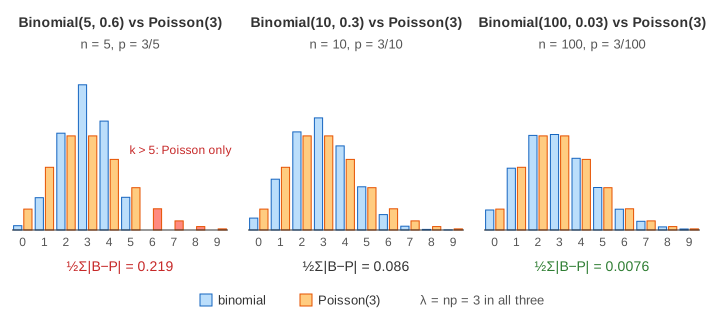
P(X = k) → e^(−λ) · λ^k / k! (Poisson, mean = variance = λ)This is the Poisson limit theorem, also called the law of rare events (Demo: n → ∞ with λ = 3 steps n through 5, 10, 20, 50, 100).
How close is close
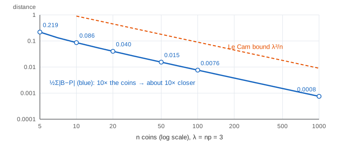
The page measures the gap as the total variation distance d = ½Σk|B(k) − P(k)|: the largest difference in probability the two models can give any event.
| n | p = 3/n | variance np(1−p) | B(3) | P(3) | d |
|---|---|---|---|---|---|
| 5 | 0.6 | 1.20 | 0.3456 | 0.2240 | 0.219 |
| 10 | 0.3 | 2.10 | 0.2668 | 0.2240 | 0.086 |
| 20 | 0.15 | 2.55 | 0.2428 | 0.2240 | 0.040 |
| 50 | 0.06 | 2.82 | 0.2311 | 0.2240 | 0.015 |
| 100 | 0.03 | 2.91 | 0.2275 | 0.2240 | 0.0076 |
Ten times the coins gives about ten times closer. Le Cam's inequality makes this precise: d ≤ np² = λ²/n. A common rule of thumb is to use Poisson for a binomial when n ≥ 20 and p ≤ 0.05.
Mean and variance
Both models have mean λ. The binomial variance np(1−p) = λ(1 − p) is smaller than Poisson's λ, so for a large p the binomial is narrower and taller: 2.10 against 3 at n = 10, 2.91 against 3 at n = 100 (Demo: mean and variance). "Variance equals mean" is a quick test of whether count data look Poisson.
Where the approximation breaks
With n = 5 and λ = 3 each coin lands heads 60% of the time: these are not rare events. Five coins can give at most 5 heads, yet Poisson(3) puts P(X > 5) = 0.0839 on 6 or more (Demo: p too big, Poisson spills past n). For a large p, the normal distribution with mean np and variance np(1−p) is the better approximation, as the central limit theorem predicts.
Where Poisson counts show up
Any count of many independent chances that are each unlikely: requests to a server per second, typos per page, calls to a help desk per minute, radioactive decays per second. One person in 100 clicking an ad is Binomial(100, 0.01), and with λ = 1 it is already within 0.003 of Poisson(1) (Demo: rare events, λ = 1, n = 100). The time between Poisson events follows the exponential distribution.
What the page leaves out
- Poisson processes in continuous time and the exponential waiting times between events.
- Other limits: Binomial → normal for large np(1−p), Poisson → normal for large λ.
- Coins with different probabilities pi (Le Cam's bound Σpi² still holds).
- Fitting λ to data and testing whether data are Poisson (dispersion test, chi-square).
- Counts above 12, which the chart and table do not draw.