The idea: a map of causes and effects
A Bayesian network is a directed acyclic graph where each node is a random variable and each arrow points from a cause to its effect. Each node carries a conditional probability table (CPT): the probability of the node given each combination of its parents. Together they define the whole joint distribution, with far fewer numbers than a table of every combination.
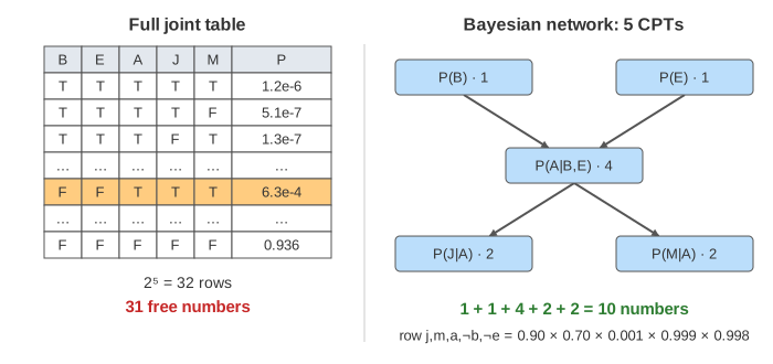
The page uses Judea Pearl's classic example, with the numbers from Russell & Norvig. You have a burglar alarm at home. A burglary or an earthquake can set it off. Your neighbours John and Mary call you at work when they hear it, but John sometimes mistakes the phone for the alarm and Mary sometimes misses it with loud music on. Set a node to true or false with its dropdown and every bar updates to P(node = true | evidence). Pick a node and press Infer to see that number computed term by term.
CPTs and the chain rule
| node | parents | P(node = true | parents) | numbers |
|---|---|---|---|
| Burglary | none | 0.001 | 1 |
| Earthquake | none | 0.002 | 1 |
| Alarm | B, E | B,E: 0.95 · B,¬E: 0.94 · ¬B,E: 0.29 · ¬B,¬E: 0.001 | 4 |
| JohnCalls | A | A: 0.90 · ¬A: 0.05 | 2 |
| MaryCalls | A | A: 0.70 · ¬A: 0.01 | 2 |
Each table stores only P(true); P(false) is 1 minus it. The chain rule writes any joint as a product of conditionals, P(B,E,A,J,M) = P(B) P(E|B) P(A|B,E) P(J|B,E,A) P(M|B,E,A,J). The network adds one assumption: each node is conditionally independent of its other predecessors given its parents. So the long conditionals shrink to the CPTs:
P(B,E,A,J,M) = P(B) P(E) P(A|B,E) P(J|A) P(M|A)

P(j, m, a, ¬b, ¬e) = 0.90 × 0.70 × 0.001 × 0.999 × 0.998 = 0.000628
With n Boolean nodes and at most k parents each, that is n·2k numbers instead of 2n − 1 (Demo 4).
Inference by enumeration
A query asks for P(X | e): the distribution of a query variable X given the observed evidence e. The other variables are hidden and must be summed out:
P(X | e) = α Σhidden P(X, e, hidden) = α Σhidden Π P(node | parents)
For P(Burglary | JohnCalls = true, MaryCalls = true) the hidden variables are E and A, so each value of B has 2 × 2 = 4 terms. Each term takes one entry from each CPT (the page highlights the rows it uses). The sums are 0.000592 for b and 0.001492 for ¬b. They are not probabilities yet, because they still include P(j, m); α = 1 / (sum of both) rescales them to add up to 1, giving P(b | j, m) = 0.284 (Demo 2). Two calls make a burglary 284 times more likely than the prior 0.001, but still less likely than not: false alarms from the 0.001 row are common because burglaries are so rare.
Enumeration takes time O(2n) for n hidden variables. Variable elimination does the same sums but caches the repeated sub-products (the P(j|a) P(m|a) part appears in every term) and is the standard exact method.
Pruning irrelevant variables
A hidden variable with no evidence below it sums to 1: Σm P(m | a) = 1 for any a. So every variable that is not the query, the evidence or one of their ancestors can be dropped before enumerating. For the prior P(Burglary), everything except B is pruned and the answer is just the CPT entry, 0.001 (Demo 1). The pruned nodes turn grey on the canvas.
Explaining away
Burglary and Earthquake are independent: P(b | e) = P(b) = 0.001. But once their common effect is observed, they compete to explain it. With both calls, P(b | j, m) = 0.284. Learn that there was an earthquake and it drops to P(b | j, m, e) = 0.003: the earthquake already explains the alarm, so a burglary is no longer needed (Demo 3). This is explaining away, the reason a common effect makes its causes dependent.
Conditional independence and d-separation
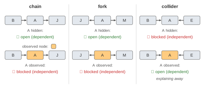
d-separation reads independences straight off the graph. Information can flow along a path unless the path is blocked. Every path is made of three kinds of connection:
| connection | example | middle hidden | middle observed |
|---|---|---|---|
| chain X → Z → Y | B → A → J | dependent | independent |
| fork X ← Z → Y | J ← A → M | dependent | independent |
| collider X → Z ← Y | B → A ← E | independent | dependent (explaining away) |
In Demo 5, John calling raises P(MaryCalls) from 0.012 to 0.040, because the fork through the hidden Alarm is open. Once Alarm = true is observed, P(MaryCalls) is 0.70 whether John called or not: JohnCalls ⟂ MaryCalls | Alarm. A collider is opened by observing the middle node or any of its descendants, which is why the two calls in Demo 3 are enough to make Burglary and Earthquake compete.
Beyond enumeration
Exact inference in a general network is NP-hard, so large networks use variable elimination with a good order, the junction tree algorithm, or approximate methods such as likelihood weighting and Gibbs sampling. A Naive Bayes classifier is the simplest Bayesian network: one class node with every feature as a child, so the features are independent given the class. An HMM is a Bayesian network unrolled over time.
Bayes' Theorem shows a single update (prior to posterior) on a medical test before you chain many of them through a network.
What the page leaves out
Variables with more than two values, continuous variables, variable elimination and junction trees, sampling methods, learning the CPTs or the structure from data, and causal interventions (do-calculus). The bars are computed by summing the full 32-row joint, which only works for tiny networks.