The idea: estimate a probability by counting samples
Exact inference in a Bayesian network sums over every assignment of the hidden variables, which takes exponential time in large networks. Sampling gives up exactness: generate many random assignments that follow the network's distribution, then count how often the query is true. The more samples, the closer the count gets to the true probability.
The page uses the sprinkler network from Russell & Norvig. Clouds make rain likely and make the sprinkler less likely to be on; either one can wet the grass.
| node | parents | P(node = true | parents) |
|---|---|---|
| Cloudy (C) | none | 0.5 |
| Sprinkler (S) | C | C: 0.1 · ¬C: 0.5 |
| Rain (R) | C | C: 0.8 · ¬C: 0.2 |
| WetGrass (W) | S, R | S,R: 0.99 · S,¬R: 0.90 · ¬S,R: 0.90 · ¬S,¬R: 0.0 |
To draw a variable, the page takes a random number u between 0 and 1 and sets the variable to true when u is below its CPT entry. Pick a method and a query, then press Draw 1 Sample to see each node drawn, or Draw 100 Samples to watch the estimate bar and the chart approach the exact answer (the green mark, computed by enumeration).
Rejection sampling
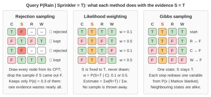
Prior sampling visits the nodes in topological order (parents first) and draws each one from the CPT row that matches its parents' values. The result is one sample from the full joint distribution. Rejection sampling adds one rule: if the sample disagrees with the evidence, throw it away. The kept samples are then distributed exactly as P(· | e), so
P(X = true | e) ≈ (kept samples with X = true) / (kept samples)
The page stops a sample as soon as an evidence node comes out wrong, since nothing drawn later can save it (Demo 1). For P(Rain | Sprinkler = T), about 30% of samples survive, because P(Sprinkler = T) = 0.3; after 500 samples the estimate is close to the exact 0.300 (Demo 2).
The weakness is waste. The fraction kept is P(e), and P(e) shrinks exponentially with the number of evidence variables. For P(Cloudy | Sprinkler = T, Rain = T, WetGrass = F) the evidence has probability 0.0009: rejection keeps about one sample in 1,100, and 500 samples give no estimate at all (Demo 3).
Likelihood weighting
Likelihood weighting never draws the evidence variables. It fixes them to their observed values and draws only the others. To make up for forcing the evidence, each sample gets a weight: the product of P(ei | parents) over the evidence variables, using the parents' values in this sample.
w = Πevidence P(ei | parents(Ei))
P(X = true | e) ≈ Σ w(samples with X = true) / Σ w(all samples)
On the rare evidence, only Cloudy is drawn. A sample with C = T gets w = 0.1 × 0.8 × 0.01 = 0.0008 and one with C = F gets w = 0.5 × 0.2 × 0.01 = 0.001. Every sample counts, and the weighted estimate settles near the exact 0.444 (Demo 4). The catch is weight degeneracy: when evidence sits below the variables being drawn (like WetGrass here), the samples are drawn without looking at it, and a few samples with large weights can dominate the sum.
Gibbs sampling and the Markov blanket
Gibbs sampling is a Markov chain Monte Carlo (MCMC) method. It keeps one complete state: the evidence at its observed values, the other variables set at random. Each step picks the next non-evidence variable and redraws it given the current values of everything else. Only the variable's Markov blanket matters: its parents, its children and its children's other parents.
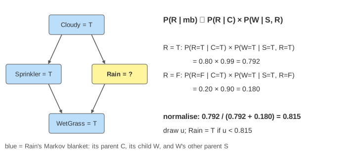
P(x | mb(X)) ∝ P(x | parents(X)) × Πchildren Y P(y | parents(Y))
Each new state is one more sample, and the fraction of states with X = true estimates the posterior. The states form a Markov chain whose long-run distribution is P(· | e), so the estimate converges, but neighbouring states are strongly correlated: they differ in at most one variable. In Demo 5, 404 steps for P(Rain | Sprinkler = T, WetGrass = T) land near the exact 0.320. See Markov Chains for why a chain settles into a stationary distribution.
Which method, and how many samples?
| method | evidence | wasted samples | weak spot |
|---|---|---|---|
| rejection | drawn, then checked | 1 − P(e) | rare evidence |
| likelihood weighting | fixed, weighted | none | evidence far down the network, uneven weights |
| Gibbs | fixed | none | correlated states, slow mixing with near-deterministic CPTs |
For independent samples the error shrinks like 1/√N, the same rate as in Monte Carlo estimation of π and the law of large numbers: four times as many samples halve the error. The convergence chart on the canvas shows the early wobble flattening out.
What the page leaves out
Burn-in and thinning for Gibbs, random-order and blocked Gibbs, Metropolis–Hastings, importance sampling with better proposals, particle filters for networks over time, and variables with more than two values.