Particle Filter Visualization | Predict, Weight by Sensor, Resample

The idea: guess with many samples

A robot drives along a corridor with three doors and does not know where it is. Its only sensor says "door" or "wall". A particle filter keeps many guesses of the position at once. Each guess is a particle: a position x and a weight w. Where the particles crowd, the robot probably is. The share of the weight in an interval is the filter's probability that the robot is there. This collection of guesses is the belief.

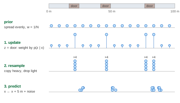
Four rows of dots over a corridor with three doors. Prior: 16 dots spread evenly. Update with z = door: dots at the doors get tall weight stems, the others short. Resample: four copies stacked at each door dot, the others gone. Predict: the copies move 5 m right and spread a little — One cycle: weight by the sensor, copy the heavy guesses, then move every guess like the robot.

Press Sense, Resample and Move to run the cycle one phase at a time, or pick a demo and press Run Demo. The top panel is the true world, which the filter never sees. The middle panel draws one dot per particle; its height is the weight times N, so 1 means "an average particle". The bottom panel adds the weights up in 5 m bins.

One cycle: predict, update, resample

Predict (motion model). The robot was told to drive u = +5 m. Every particle moves the same way, plus random noise: x ← x + 5 + ε, with ε drawn from a normal distribution with σ = 1 m. The noise spreads the cloud: moving makes the robot less sure where it is.
Update (sensor model). The sensor reads z. Each weight is multiplied by p(z | x), how likely that reading is if the robot were at the particle's position, and then all weights are divided by their sum. On this page p(door | door) = 0.9, p(wall | door) = 0.1, p(door | wall) = 0.05 and p(wall | wall) = 0.95.
Resample. Draw N new particles, each one a copy of an old particle chosen with probability equal to its weight. Heavy particles get several copies, light ones vanish, and every weight goes back to 1/N. The page uses systematic resampling: one random offset r in [0, 1/N), then N evenly spaced pointers r, r + 1/N, … over the running sum of the weights.

This is Bayes' rule, done with samples. Predict computes the prior p(x_t | z_1..t−1), update multiplies by the likelihood p(z_t | x_t) and normalizes, as in Bayes' Theorem. Because the belief is a set of samples, any motion model and any sensor model work, however nonlinear (Demo: one cycle, step by step).

Three clumps, and a misleading mean

At t = 0 the particles are spread evenly. The robot stands at door 1 and reads "door". All three doors fit that reading, so after the update the weight sits in three clumps of about 30% each. The effective sample size drops from 50 to 16.4 (see below). The weighted mean is 48.7 m, next to door 2, while the robot is at 20 m.

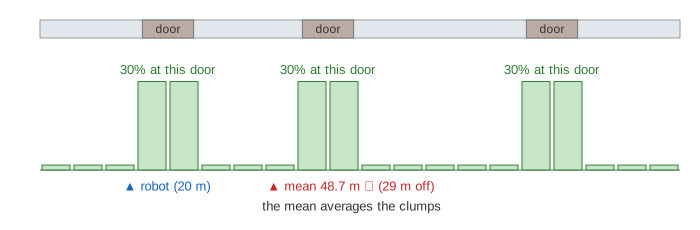
Belief histogram after the first door reading: three equal bumps of about 30 percent at the three doors. The robot is at 20 m under the first bump; the mean, 48.7 m, is under the middle bump, 29 m off — After one "door" the belief has three peaks; a single number such as the mean hides that.

The belief is multimodal, and a particle filter can hold it as it is. A Kalman filter cannot: it keeps a single Gaussian. Moving and sensing again breaks the tie. Only a robot that started at door 1 sees "door" again 25 m later; a robot at door 2 would see a wall there, and a robot at door 3 would be past the end of the corridor. After 8 cycles the robot is at 60 m and the mean is 61.2 ± 4.7 m (Demo: global localization).

Why resample: weight degeneracy

Without resampling, every update multiplies the weights again. A few particles that happened to agree with every reading end up with almost all of the weight, and the rest are wasted computing positions that no longer matter. The effective sample size N_eff = 1 / Σ w_i² measures this: it equals N when all weights are equal and 1 when one particle has all the weight. With 6 updates and no resampling it falls from 50 to 9.2, so the filter works like one with 9 particles (Demo: no resampling, the weights degenerate).

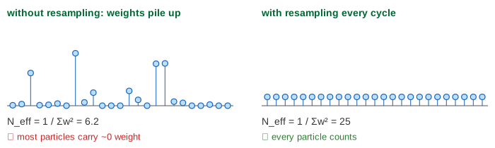
Left: 25 weight stems, a few tall and most near zero, N_eff = 6.2. Right: 25 equal short stems after resampling, N_eff = 25 — Resampling moves the effort onto the guesses that still matter; N_eff shows how many particles are really working.

Resampling has a cost too. It throws away diversity: after it, several particles sit on exactly the same spot, and only the motion noise of the next predict spreads them again. Many libraries therefore resample only when N_eff falls below a threshold such as N / 2.

The kidnapped robot

Once the filter has converged, every particle is near one place. If someone now carries the robot 18 m back (from 30 m to 12 m), no particle is near the truth. Updates can only reweight existing particles, so the cloud keeps tracking its own wrong position: 7 cycles later the robot is at 47 m and the mean at 69.1 m (Demo: kidnapped robot, plain resampling).

The common fix is to replace a small share of the particles with random positions at every resample. Most random guesses die at once, but the ones that land near the robot agree with its readings and grow into a new clump. With 10% random particles, about three quarters of the weight is back within 5 m of the robot after 7 cycles (Demo: kidnapped robot, 10% random particles). The price is a slightly wider belief even when nothing goes wrong.

Particle filter, Kalman filter, grid filter

filter	belief is	multimodal?	cost per step
Kalman filter	one Gaussian: mean and covariance	no	small matrix products
Grid (histogram) filter	a probability per cell	yes	grows with the number of cells, so with the size of the space
Particle filter	N weighted samples	yes	O(N), with N set by how much accuracy you need

The particle filter is a sequential Monte Carlo method: like Monte Carlo π, it trades exact formulas for random samples. The hidden position that changes step by step is the same set-up as a hidden Markov model, where the Viterbi algorithm finds the most likely path; see Markov Chains for the motion part alone.

What the page leaves out

Two and three dimensions with heading (real Monte Carlo localization uses x, y and θ and a laser scan), sensors with continuous readings, adaptive particle counts (KLD sampling), resampling only when N_eff is low, augmented MCL that injects random particles only when the readings stop fitting, and particle filters for other problems such as tracking and SLAM.