The idea: one rule, bounded or not
Pick a complex number c. Start at z₀ = 0 and apply one rule again and again:
zₙ₊₁ = zₙ² + c z₀ = 0, z₁ = c, z₂ = c² + c, z₃ = (c² + c)² + c, …The list z₀, z₁, z₂, … is the orbit of 0. For some c it stays in a small region for ever; for others it runs off to infinity. The Mandelbrot set is the set of all c whose orbit stays bounded. Each pixel of the picture is one c; the set is the dark shape.
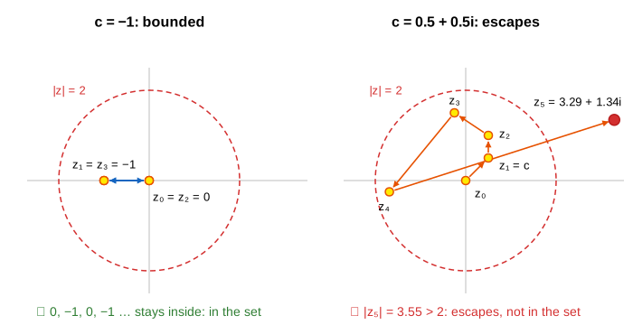
Pick a c in the orbit of c menu to draw its orbit on top of the set. (Demo: orbit of c = −1: period 2, bounded, Demo: orbit of c = 0.3: escapes after 12 steps.) Squaring a complex number squares its length and doubles its angle (see Complex Numbers: add, multiply, rotate), so the orbit swings around the origin as well as in and out.
The escape test: why 2
You cannot run an orbit for ever, so the computer needs a test that says "this one will escape". The test is |z| > 2. If |c| ≤ 2 and some |zₙ| > 2, then
|zₙ₊₁| = |zₙ² + c| ≥ |zₙ|² − |c| ≥ |zₙ|² − |zₙ| = |zₙ|·(|zₙ| − 1) > |zₙ|and the factor |zₙ| − 1 > 1 keeps growing, so |z| goes to infinity. (If |c| > 2, already |z₂| = |c² + c| ≥ |c|(|c| − 1) > |c| and the same argument applies.) So the whole set lies inside the disk |c| ≤ 2, and an orbit that ever leaves the circle |z| = 2 is gone for good.
| c | orbit | verdict |
|---|---|---|
| 0 | 0, 0, 0, … | in: a fixed point |
| −1 | 0, −1, 0, −1, … | in: period 2 |
| −2 | 0, −2, 2, 2, 2, … | in: the tip of the set, on the circle |
| i | 0, i, −1 + i, −i, −1 + i, −i, … | in: a boundary point |
| 0.3 | 0.3, 0.39, 0.452, … 1.376, 2.193 | out: escapes at step 12 |
| 0.5 + 0.5i | 0.5 + 0.5i, 0.5 + i, −0.25 + 1.5i, −1.69 − 0.25i, 3.29 + 1.34i | out: escapes at step 5 |
Colouring by escape count, and the iteration budget
For each pixel the page runs the rule until |z| passes the bail-out radius or a step limit, the iteration budget. Pixels that never escape are painted dark: as far as the budget can tell, they are in the set. The rest are coloured by how many steps they took. A plain step count gives stripes; the page uses the smooth escape count
μ = n + 1 − log₂(ln |zₙ|) (run on to |z| > 1000 so the correction is accurate)which slides continuously from one count to the next, and maps √μ onto a colour cycle. Points far from the set escape in 1–3 steps (pale); points near its edge take hundreds or thousands (the bands).
The budget matters. A point that would escape at step 900 looks like a member of the set if you stop at 500. So with too few iterations the edge looks fat and smudged, and zooming in needs more and more of them. The auto setting uses 100 + 90 per halving of the view width (about 3800 at 10⁻¹²). (Demo: too few iterations: 100 vs 1000 (Seahorse Valley): at width 0.0117 the black share drops from about 21% to 3% as the budget rises.)
The main cardioid and the period-2 disk
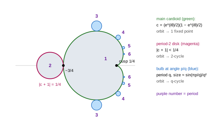
The big heart-shaped body is the main cardioid. For c inside it, the orbit settles on one attracting fixed point z* = z*² + c. The fixed point attracts when the slope of z ↦ z² + c there is less than 1 in size, |2z*| < 1. Put z* = e^(iθ)/2 on the edge of that condition and solve for c:
c = z* − z*² = (e^(iθ)/2)·(1 − e^(iθ)/2) θ from 0 to 2πThat curve is the cardioid, the green overlay. Its cusp is c = 1/4 (θ = 0) and its leftmost point is c = −3/4 (θ = π). The same is done for 2-cycles: the orbit alternates between two points, and the cycle attracts exactly when |c + 1| < 1/4, the magenta disk to the left of the cardioid. It touches the cardioid at −3/4. (Demo: the set, its main cardioid and period-2 disk.) These closed forms are also a speed trick: the page skips the loop for every pixel inside them.
Bulbs and their periods
Around the cardioid sits a ring of round bulbs. The bulb attached at angle θ = 2π·p/q (in the cardioid formula) has period q: for c inside it, the orbit ends in a cycle of q points that it visits in turn. The disk is the p/q = 1/2 bulb (period 2); the big bulbs at the top and bottom are 1/3 and 2/3 (period 3); then 1/4 and 3/4 (period 4), and so on. A bulb of period q has a size of about sin(πp/q)/q², so the bulbs shrink fast. Turn the overlay on to see the periods written next to the bulbs. (Demo: orbit of c = −0.12 + 0.75i: period 3: the orbit visits three points in turn.) The same doubling of periods you see from the cardioid (period 1) to the disk (period 2) and on along the real axis is the period-doubling cascade of the Logistic Map: on the real line, z² + c and r·x(1 − x) are the same map after a change of variables.
Connected, with copies everywhere
The thin filaments that leave the bulbs look broken at low resolution, but the set is connected: one piece, with no islands (Douady and Hubbard, 1982). The dark specks you meet when zooming are joined to the main body by filaments too thin for any pixel.
Zoom in almost anywhere on the edge and you find mini copies of the whole set, each with its own cardioid, disk and bulbs. On the needle to the left, around −1.7685, sits the period-3 copy: its points have period-3 orbits. (Demo: a mini-Mandelbrot on the real axis.) The edge never becomes smooth: its fractal dimension is 2, the most a curve in the plane can have (Shishikura, 1998). Different regions have their own look: Seahorse Valley between the cardioid and the disk (Demo: zoom into Seahorse Valley), Elephant Valley at the cusp 0.25.
Each c also has its own picture: the Julia set of z ↦ z² + c, the starting points z₀ whose orbits stay bounded for that fixed c. It is connected exactly when c is in the Mandelbrot set. See Julia Sets.
Zooming, and where double precision stops
Play: dive halves the view width 41 times, from 3 down to 3/2⁴¹ ≈ 1.4·10⁻¹², a zoom of about 2·10¹². If the final view filled a 20 cm screen, the whole set at that scale would be about three times the distance from the Earth to the Sun. The spirals keep coming.
The page computes with ordinary 64-bit double precision numbers, which carry 53 bits, about 16 significant digits. Near |c| ≈ 0.74 neighbouring doubles are 2⁻⁵³ ≈ 1.1·10⁻¹⁶ apart (see IEEE 754 Floating Point). A 660-pixel view of width w has pixels w/660 wide: about 14 doubles at w = 10⁻¹², only about 1.4 at w = 10⁻¹³. Below that, neighbouring pixels start to get the same c and the picture turns to blocks. (Demo: past the limit: width 10⁻¹⁴, pixels turn to blocks.) Deep-zoom programs go further with arbitrary-precision numbers, or with perturbation theory: one orbit in high precision, the pixels as small doubles relative to it.
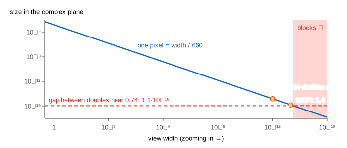
| view width | zoom | pixel (660 px) | doubles per pixel near 0.74 |
|---|---|---|---|
| 3 | ×1 | 4.5·10⁻³ | 4·10¹³ |
| 10⁻⁶ | ×3·10⁶ | 1.5·10⁻⁹ | 1.4·10⁷ |
| 1.4·10⁻¹² | ×2·10¹² | 2.1·10⁻¹⁵ | 19 |
| 1.1·10⁻¹⁴ | ×2.8·10¹⁴ | 1.6·10⁻¹⁷ | 0.15: blocks |
Each picture is computed once into an off-screen image and cached, and the line under the picture shows its size and how long it took. While Playing the page renders at 220 × 220 pixels to keep each frame quick. A deep view costs thousands of steps per pixel, so the page first measures the average on a small sample and picks the number of pixels that keeps a picture under about a second (about 380 × 380 at the end of the dive).
Other fractals built from a simple rule: Fractal Curves (Koch, Hilbert and dragon curves by replacement), The Chaos Game (random jumps that draw the Sierpiński triangle), and the Weierstrass Function, a graph with detail at every scale.
What the page leaves out
Free zooming by clicking (the page zooms toward four fixed places, so every demo is repeatable), arbitrary precision and perturbation theory (the floor is about 10⁻¹³), distance estimation and other colouring methods, the exact count of hyperbolic components, external rays and the combinatorics of which bulb hangs where, the Julia sets themselves (see the Julia Sets page), the area of the set (about 1.5066, known only numerically), and higher powers z ↦ z^d + c (the "Multibrot" sets).