The idea: one simple rule, repeated
Take a number x between 0 and 1, compute r·x·(1 − x), and feed the answer back in:
xₙ₊₁ = r · xₙ · (1 − xₙ) x₀ = 0.2, 2.5 ≤ r ≤ 4This is the logistic map. It started as a toy model of a population: x is the population as a fraction of the most the land can hold, r is the growth rate, and the factor (1 − x) slows growth when the land fills up. Depending on r, the sequence x₀, x₁, x₂, … settles on one value, bounces between 2, 4, 8 … values, or never settles at all.
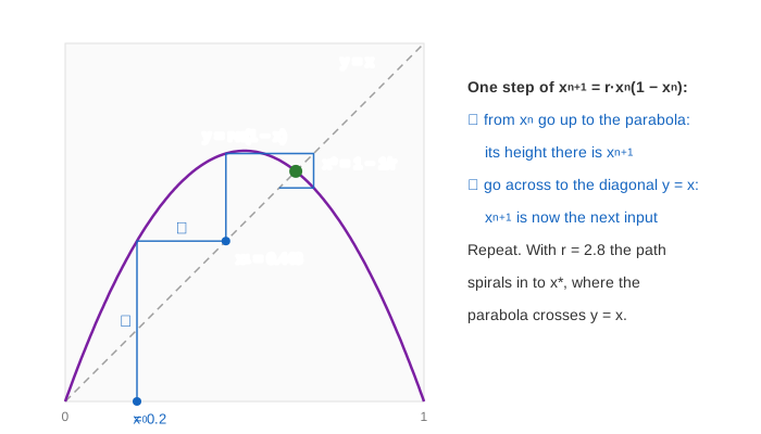
The cobweb plot
The left plot draws the rule as the parabola y = r·x(1 − x). One step of the map is two strokes of the pen: up (or down) from xₙ to the parabola, which gives the height xₙ₊₁, then across to the diagonal y = x, which moves that height back onto the x scale so it can be the next input. The page draws 50 such steps from x₀ = 0.2, and the same 50 values as a time series xₙ against n below it. (Demo: r = 2.8, the cobweb spirals into x* draws the first 4 steps one at a time with their numbers.)
The top of the parabola is at x = ½, with height r/4. For r ≤ 4 that is at most 1, so x never leaves [0, 1]. For r > 4 it would, and the orbit escapes to −∞.
The fixed point and its slope
A fixed point is an x the map leaves alone: x = r·x(1 − x). Besides x = 0 the answer is
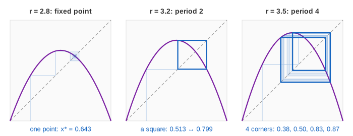
x* = 1 − 1/r r = 2.5: 0.6 r = 2.8: 0.643 r = 3.2: 0.688On the cobweb it is where the parabola crosses y = x (the green dot). Whether the orbit goes there depends on the slope of the map at x*: near x*, each step multiplies the distance to x* by f′(x*) = r(1 − 2x*) = 2 − r. If |2 − r| < 1, that is 1 < r < 3, the distance shrinks and x* is stable; the slope is negative for r > 2, so the orbit lands on alternate sides and the cobweb spirals in. At r = 3 the slope reaches −1, and for r > 3 the fixed point pushes the orbit away (the red ring). This is the same test as for Newton's method, which is also a map iterated to its fixed point; Newton's map has slope 0 at the root, which is why it converges so fast.
Period doubling and Feigenbaum's δ
Past r = 3 the orbit does not run off; it settles on a 2-cycle: two values a and b with f(a) = b and f(b) = a. On the cobweb that is a square around x*. The 2-cycle is stable until r = 1 + √6 ≈ 3.449, where it splits into a 4-cycle, which splits into an 8-cycle, and so on: the period-doubling cascade (Demo: period doubling 1 → 2 → 4 → 8 → 16).
| period becomes | at r | gap to the previous | ratio of gaps |
|---|---|---|---|
| 2 | 3 | ||
| 4 | 1 + √6 ≈ 3.4495 | 0.4495 | |
| 8 | 3.5441 | 0.0946 | 4.75 |
| 16 | 3.5644 | 0.0203 | 4.66 |
| 32 | 3.5688 | 0.0044 | 4.67 |
| ∞ (chaos) | r∞ ≈ 3.5699 | → δ ≈ 4.669 |
Each gap is about 4.669 times shorter than the one before. That number, Feigenbaum's constant δ ≈ 4.6692, is not special to this parabola: every smooth map with one hump doubles its period at the same rate. Because the gaps shrink geometrically, infinitely many doublings fit before r∞ ≈ 3.5699.
Chaos and the bifurcation diagram
Past r∞ most values of r give no cycle at all: the orbit wanders forever without repeating. That is chaos: a rule with no randomness in it, whose output looks random. The right plot, the bifurcation diagram, shows all of this at once. For each r (one column per pixel) the page runs 300 steps from 0.2 to forget the start, then plots the next 100 values. A stable fixed point is one dot per column, a 2-cycle two dots, and chaos a smear of dots. The red line marks the current r, and the red dots on it are 64 of its values after 5000 steps: the same values the cobweb ends up circling. (Demo: build the bifurcation diagram, r 2.5 → 4, or press Play r 2.5 → 4: each step adds 0.01 to r, the next columns appear and the cobweb changes with them.)
Zoom into a piece of the chaotic part and the same tree of splitting branches appears again, smaller: the diagram is self-similar, like the graph of the Weierstrass function. At r = 4 the parabola reaches 1 and the orbit covers all of [0, 1] (Demo: r = 4, full chaos).
The period-3 window
The chaotic region has white gaps: windows where a stable cycle comes back. The widest one opens at r = 1 + √8 ≈ 3.8284 with a 3-cycle; at r = 3.83 the orbit visits 0.156, 0.505, 0.957 in turn. Just below 3.8284 the orbit looks like period 3 for long stretches and then breaks out in a burst of chaos (intermittency). Inside the window the 3-cycle doubles to 6 at about 3.8415, then to 12, 24, …, and chaos returns at about 3.85. (Demo: r = 3.83, the period-3 window.)
Sensitive to the start
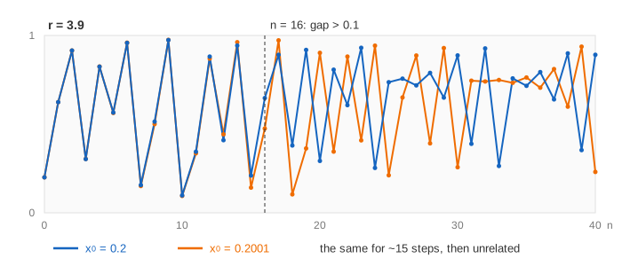
Turn on the second start x₀ = 0.2001 and the time series gets a second, orange line. When r gives a stable cycle, both starts end on the same cycle and the gap dies out. In chaos the gap grows by roughly the same factor every step: at r = 3.9 the two lines agree for about 15 steps, then the gap passes 0.1 at n = 16 and the two have nothing to do with each other. (Demo: r = 3.9, chaos: starts 0.2 and 0.2001.) This is sensitive dependence on initial conditions: since x₀ is never known exactly, long-range prediction is impossible even though every step is exact.
Summary
| r | long run from x₀ = 0.2 |
|---|---|
| 1 < r < 3 | the fixed point x* = 1 − 1/r (2.8: 0.643) |
| 3 < r < 3.449 | period 2 (3.2: 0.513, 0.799) |
| 3.449 < r < 3.544 | period 4 (3.5: 0.383, 0.501, 0.827, 0.875) |
| 3.544 … 3.5699 | period 8, 16, 32, … |
| 3.5699 < r ≤ 4 | chaos, with windows such as period 3 from 3.8284 |
The logistic map is the step-by-step cousin of the logistic growth equation dP/dt = kP(1 − P/M), which Euler's method solves in small steps; the smooth equation always settles, and the chaos here comes from taking steps as large as a whole generation. Other iterations that settle on a fixed point are bisection, Newton and the secant method and the distribution of a Markov chain.
More simple rules applied again and again: on the real line z² + c is the logistic map in disguise, and its period doubling runs along the needle of The Mandelbrot Set; the same z → z² + c in the complex plane draws Julia sets; a weather model takes the road to chaos in three dimensions in The Lorenz Attractor; and the 3n + 1 rule grows a seaweed tree in The Collatz Conjecture.
What the page leaves out
r below 2.5 (0 < r < 1: the population dies out; 1 < r < 2: x* is reached without overshooting) and r above 4 (the orbit escapes); the second fixed point x = 0; the formulas for the 2-cycle; Lyapunov exponents, which measure the growth rate of the gap; Sharkovskii's theorem ("period 3 implies all periods"); the Mandelbrot set, which is the same map for complex numbers; and zooming into the diagram. The diagram uses x₀ = 0.2 and 300 + 100 steps per column, so columns very close to a doubling point have not fully settled.