The idea: three short equations, one butterfly
In 1963 the meteorologist Edward Lorenz studied three equations for a point (x, y, z) moving in space:
dx/dt = σ(y − x)
dy/dt = x(ρ − z) − y        σ = 10,  β = 8/3,  ρ = 28
dz/dt = xy − βz
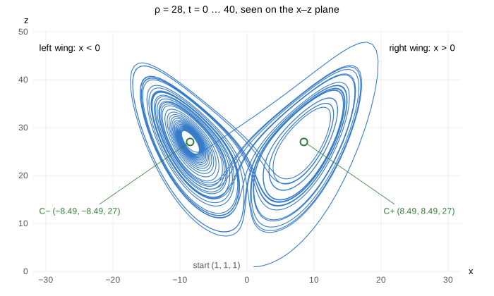
There is no randomness anywhere: the same start always gives the same path. Yet at ρ = 28 the path never settles down and never repeats. It loops around one "wing", then the other, and switches in a pattern that looks random. The shape it traces is the Lorenz attractor, the famous butterfly.
Where it comes from: a weather model cut down to 3 numbers
Lorenz started from the equations of a layer of air heated from below, which rolls over in convection cells. He kept only three numbers: x is how fast the roll turns, y is the temperature difference between the rising and the falling side, and z is how far the temperature profile is bent away from a straight line. The constants are physical too: σ (the Prandtl number) compares how fast the air loses momentum and heat, β is set by the shape of the cell, and ρ (the Rayleigh number, scaled) says how strongly the layer is heated.
The story he told: to repeat a run, he typed in numbers from a printout that had been rounded from 6 digits to 3. The new run matched the old one for a while and then went somewhere completely different. A difference of 0.000127 was enough. His 1972 talk was titled Does the flap of a butterfly's wings in Brazil set off a tornado in Texas?, and the name stuck.
The fixed points C±
A fixed point is a place where all three rates are 0, so a path that starts there stays there. σ(y − x) = 0 gives y = x; xy = βz gives z = x²/β; and x(ρ − z) − y = 0 then gives x² = β(ρ − 1). So besides the origin there are two:
C± = ( ±√(β(ρ − 1)), ±√(β(ρ − 1)), ρ − 1 ) ρ = 28: (±8.49, ±8.49, 27)They are the green rings on the canvas, the centres of the two wings. A path spirals around one of them, but at ρ = 28 the spiral grows outward, and when it is wide enough the path is thrown over to the other side. That is the wing switch you see in the x(t) chart: x > 0 on the right wing, x < 0 on the left, and no pattern in how many loops it makes before switching (Demo: ρ = 28, trace the butterfly: 17 switches by t = 40).
Sensitive dependence: two starts 0.001 apart
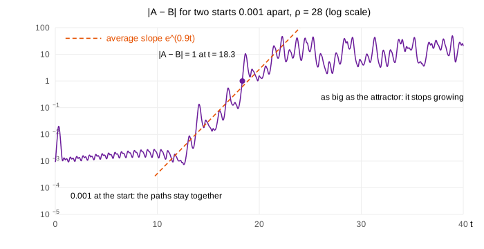
Turn the second start on: B starts at (1.001, 1, 1), 0.001 from A. For a while the red and blue paths lie on top of each other. Then they come apart and follow unrelated paths (Demo: two starts 0.001 apart separate (ρ = 28): |A − B| passes 1 at t ≈ 18.3).
The chart on the right shows |A − B| on a log scale. On a log scale an exponential e^(λt) is a straight line, and that is what you see: the error grows on average like
|A − B| ≈ 0.001 · e^(λt), λ ≈ 0.9 per time unitλ is the largest Lyapunov exponent. Every 0.77 time units the error doubles, every 2.6 it grows ten times. The growth is bumpy (some parts of the attractor stretch more than others), so the dashed e^(0.9t) line is an average slope. It stops when |A − B| is as big as the attractor itself, about 20: then the two points are simply at unrelated places on the butterfly.
This is why weather forecasts run out after one or two weeks. The equations can be perfect and the computer exact: any error in the starting state, however small, grows until the forecast is no better than a guess. Making the error 1000 times smaller only buys ln(1000)/0.9 ≈ 7.7 more time units. Deterministic (the future is fixed by the present) is not the same as predictable (we can work it out from what we can measure).
What ρ does
| ρ | what the path from (1, 1, 1) does | two starts 0.001 apart |
|---|---|---|
| ρ < 1 | falls into the origin: the air does not roll | come together |
| 10 | spirals into C+ = (4.90, 4.90, 9): a steady roll | come together, |A − B| → 10⁻¹³ |
| 24 | C± still pull in paths close to them, but this start spirals out from C− and joins the chaotic set | apart at t ≈ 37 |
| 24.74 | C± stop pulling paths in: long slow spirals, then chaos | apart at t ≈ 24.5 |
| 28 | the butterfly: chaos | apart at t ≈ 18.3 |
| 100 | a periodic window: a closed loop with 3 turns | stay close (~0.01) |
| 160 | a periodic orbit with 4 turns, 2 on each wing | stay close (~0.02) |
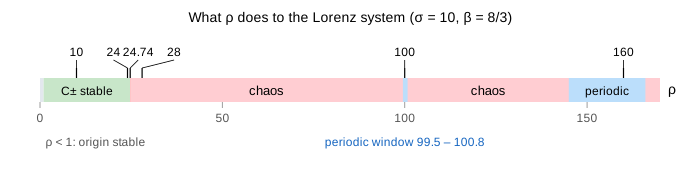
Below about 24.74 the fixed points are stable: nearby paths spiral into them (Demo: ρ = 10 spirals into a fixed point). At ρ_H = σ(σ + β + 3)/(σ − β − 1) ≈ 24.74 they lose stability (a Hopf bifurcation) and the chaotic attractor is all that is left. Between 24.06 and 24.74 both exist at once, so the long-run behaviour depends on the start (Demo: near the transition, ρ = 24 then 24.74). Much higher, chaos gives way again to stable loops in windows such as 99.5 < ρ < 100.8 and 145 < ρ < 166 (Demo: ρ = 100, a periodic window, Demo: ρ = 160, a periodic orbit). On a stable loop, two nearby starts do not run apart: chaos is what makes the error grow, not the equations being nonlinear.
The same road from order to chaos, with periodic windows inside the chaos, shows up in a one-line formula on The Logistic Map: from a Fixed Point to Chaos. A double pendulum is a chaotic system you can build on a desk.
A strange attractor
Set the view to rotating (Demo: turn the attractor). The two wings are thin, slightly tilted sheets. Paths from almost any start are pulled onto them, which is why it is called an attractor; volumes in (x, y, z) shrink by the factor e^(−(σ + 1 + β)t) ≈ e^(−13.7t), so everything ends up on a set of zero volume. But on the attractor paths stretch apart (λ ≈ 0.9) and are folded back where the wings meet. Stretch and fold, again and again, and the sheets become infinitely many sheets packed together: a fractal with dimension about 2.06, a bit more than a surface. An attractor like this is called strange. (Self-similar fractal shapes are on Fractal Curves.)
How the page computes the path
There is no formula for x(t), so the path is computed step by step with the classical Runge–Kutta method (RK4) and a fixed step dt = 0.01: 4000 steps for t = 0 to 40, for each start. Every step has an error of order dt⁵, and chaos amplifies those errors too: a different dt gives a different path after t ≈ 20 (dt = 0.005 and dt = 0.01 are more than 1 apart from t ≈ 21). The attractor's shape, the fixed points and λ do not change. RK4 against the simpler Euler step: Runge–Kutta vs Euler and Euler's Method.
What the page leaves out
Other σ and β, starts other than (1, 1, 1), the unstable periodic orbits inside the attractor, the homoclinic explosion at ρ ≈ 13.93 (where transient chaos starts), the period-doubling cascades at the edges of the windows, the Lorenz map of successive z peaks, all three Lyapunov exponents (0.9, 0, −14.6) and how the dimension 2.06 is measured. The page draws t = 0 to 40 only, with one fixed step size.