Six Types of Integrals: cut, multiply, add

The idea: one recipe, six domains

Every integral on this page is built the same way. Cut the thing you integrate over into small pieces, multiply the function by the size of each piece, and add the products. As the pieces shrink, the sum settles on one number: the integral. The six types differ only in what gets cut and how a piece is measured: a length Δx on a line, a length Δs along a curve, a measure μ of a set, an area ΔA, an area with a direction (a normal N), or a volume ΔV.

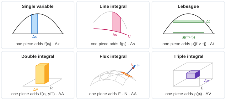
Integral	What you cut	One piece adds	The answer means
Single ∫ab f(x) dx	the interval [a, b]	f(xi) Δx	area under the curve
Line ∫C f ds	the curve C	f(pi) Δs	area of a curtain on C; mass of a wire
Lebesgue ∫E f dμ	the range of f (heights t)	μ({f > tk}) Δt	the same area, sliced sideways
Double ∬R f dA	the region R	f(xi, yj) ΔA	volume under a surface
Flux ∬S F · dS	the surface S	F · N ΔA	flow through S per second
Triple ∭E ρ dV	the solid E	ρ(pi) ΔV	mass of a solid

Every panel uses midpoint sums: the function is read at the centre of each piece. Pick n = 4, 8 or 16 pieces per direction; the panel shows the running sum Σ next to the exact value, and the narration gives the error. (Demo: all six integrals, n = 4)

1. Single variable: strips

f(x) = 4x − x² on [0, 4] is a hill of height 4. Cut [0, 4] into n strips of width Δx = 4/n; each adds f(midpoint) × Δx. With n = 4 the sum is 11.000, with 8 it is 10.750, with 16 it is 10.688, closing in on the exact 32/3 ≈ 10.667. Each doubling of n divides the error by 4 (a midpoint sum's error falls like 1/n²). (Demo: single variable, n = 4 → 8 → 16) For left, right and trapezoid sums and their errors see Riemann Sums; for why the area equals F(b) − F(a) see the Fundamental Theorem of Calculus.

2. Line integral: a curtain on a curve

Now the domain is a curve C in the floor plane: a quarter circle of radius 2 from (2, 0) to (0, 2), length π. Above each point of C stand up a wall of height f(x, y) = 1 + xy. The line integral ∫_C f ds is the area of that curtain. Cut C into n arc pieces of length Δs = π/n and add f(midpoint) × Δs: 7.246, 7.167, 7.148 for n = 4, 8, 16, against the exact π + 4 ≈ 7.142. With f = 1 the curtain has height 1 and the integral is just the length of C. (Demo: line integral, a curtain over C)

This is the scalar line integral (ds is a length). The vector line integral ∫ F · dr, where only the part of F along the path counts, gives the work done by a force: see Work Along a Path.

3. Lebesgue integral: slice the heights

Riemann cuts the x-axis. Lebesgue cuts the values of f. For each height t, look at the set where f is above t and measure it: here {f > t} is the interval (2 − √(4 − t), 2 + √(4 − t)), so its measure μ is its length 2√(4 − t). Add up μ({f > t}) × Δt over the heights:

∫ f dμ = ∫₀⁴ μ({f > t}) dt = ∫₀⁴ 2√(4 − t) dt = 32/3.

It is the same hill as panel 1 and the same number, cut the other way. (Demo: same area two ways: strips vs slabs)

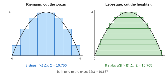
Why bother? Lebesgue's way only needs to measure sets, so it works where strips fail. The Dirichlet function (1 on rational numbers, 0 on irrational ones) has no Riemann integral on [0, 1]: every strip contains both kinds of points. But the set where it is 1, the rationals, has measure 0, so its Lebesgue integral is 0. Measures also need not be lengths: with a probability measure, ∫ X dP is the expected value of a random variable X. Limits behave better too (the monotone and dominated convergence theorems), which is why probability theory and Fourier analysis are written with Lebesgue integrals.

4. Double integral: boxes under a surface

f(x, y) = 4 − (x² + y²)/2 is a surface over the square R = [0, 2]². Cut R into n × n small squares of area ΔA = (2/n)²; over each, stand a box of height f(centre). The boxes add up to 10.750, 10.688, 10.672 for n = 4, 8, 16, tending to the volume 32/3. (Demo: double integral, boxes n = 4 → 8) Adding the boxes row by row is an iterated integral (Fubini): see Earthwork Volume and Probability Over a 2-D Region.

5. Flux integral: only the part across counts

A flux integral measures how much of a vector field F flows through a surface S. The surface here is the dome z = 2 − (x² + y²)/2 over [−1, 1]², and F = (x, 0, 1) blows up and outward along x. Cut S into patches. A patch over a small square ΔA has the vector area N ΔA, where N = (−∂z/∂x, −∂z/∂y, 1) = (x, y, 1) is perpendicular to S. Only the part of F along N goes through, so each patch adds

F · N ΔA = (x · x + 0 · y + 1 · 1) ΔA = (x² + 1) ΔA.

In the middle F points straight up and the patch adds 1 × ΔA; toward x = ±1 the field and the normal lean the same way and the patch adds more. The sum is 5.250, 5.313, 5.328 for n = 4, 8, 16, against 16/3 ≈ 5.333. The blue arrows are F, the orange ones the unit normal. (Demo: flux, only F · N counts) See also Flow Rate Through a Filter Membrane and Flux Through a Closed Surface.

6. Triple integral: voxels of a solid

A cube [0, 2]³ has density ρ = 1 + z²: light at the bottom (ρ = 1), heavy at the top (ρ = 5). Cut it into n³ small cubes (voxels) of volume ΔV = (2/n)³; each adds ρ(centre) × ΔV, its mass. Because ρ depends only on z, a whole layer has one density, so the canvas fills the cube layer by layer, darker as ρ grows. The total is 18.500, 18.625, 18.656 for n = 4, 8, 16, tending to the mass 56/3 ≈ 18.667. (Demo: triple integral, layer by layer) See also Mass of a 3D Object and Volume of a 3-D Region.

How fast the sums close in

Integral	Exact	n = 4	n = 8	n = 16
Single	32/3 ≈ 10.667	11.000	10.750	10.688
Line	π + 4 ≈ 7.142	7.246	7.167	7.148
Lebesgue	32/3 ≈ 10.667	10.768	10.705	10.681
Double	32/3 ≈ 10.667	10.750	10.688	10.672
Flux	16/3 ≈ 5.333	5.250	5.313	5.328
Triple	56/3 ≈ 18.667	18.500	18.625	18.656

For the smooth functions here each doubling of n divides the midpoint error by about 4. The Lebesgue slabs are the exception: μ({f > t}) = 2√(4 − t) has an infinite slope at the top of the hill (t = 4), so its error falls more slowly, by about 2.7 per doubling.

What the page leaves out

Every function here is smooth and positive, so there is no signed area and no improper integral (see Improper Integrals). The line and flux integrals use one fixed direction and orientation; reversing C or flipping N changes the sign of the vector versions. The Lebesgue panel only uses length as the measure; the general theory (σ-algebras, measurable functions, the convergence theorems) is described, not shown. Change of variables (polar, cylindrical, spherical coordinates and their Jacobians) and the big theorems that link these integrals (Green, Stokes, Gauss) are on Circulation Along a Closed Curve and Flux Through a Closed Surface. The 3-D pictures are a fixed oblique view drawn with rectangles, so box edges are approximate.

References

OpenStax Calculus Volume 3, Chapter 5: Multiple Integration

OpenStax Calculus Volume 3, 6.2 Line Integrals

OpenStax Calculus Volume 3, 6.6 Surface Integrals (flux)

Wikipedia: Lebesgue integration