The idea: derivatives and integrals undo each other
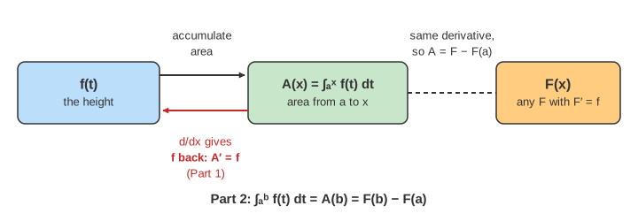
Fix a starting point a and let the right end x move. The signed area under f from a to x is then a new function of x, the area function A(x) = ∫ax f(t) dt. The Fundamental Theorem of Calculus says two things about it. Part 1: A′(x) = f(x), so the slope of the area function is the height of f. Part 2: if F is any antiderivative of f (any function with F′ = f), then ∫ab f(t) dt = F(b) − F(a). An area that would need a limit of Riemann sums comes from two values of F.
Reading the two plots
The top plot is y = f(t). The blue region is the area from a to x (orange where f is below the axis), and the red bar is the height f(x). The bottom plot is A(x), drawn as x slides right; the red line is its tangent at x. Both plots share the same x scale, marked by a grey guide line in each plot. The info panel shows f(x) and the slope of A, which is measured from A itself, and the two numbers are always equal.
| f(t) | antiderivative F(t) | A(x) = F(x) − F(a) | shape of A |
|---|---|---|---|
| 1 on [0, 4] | t | x | a straight line, slope 1 |
| t on [0, 2] | t²/2 | x²/2 | a parabola, slope = x |
| sin t on [0, 2π] | −cos t | 1 − cos x | rises to 2 at π, falls back to 0 |
| t² on [0, 2] | t³/3 | x³/3 | a cubic, ends at 8/3 |
A constant f adds the same area for every step of x, so A is a line (Demo: f = 1, A(x) = x is a line). For f = t each step adds a bit more than the last, so A curves upward: x²/2 (Demo: f = t, A(x) = x²/2).
Part 1: the sliver argument
Move x to x + Δx. The area grows by the thin strip between them: ΔA = A(x + Δx) − A(x). That strip is almost a rectangle of height f(x) and width Δx, so ΔA ≈ f(x)·Δx. Divide by Δx: ΔA/Δx ≈ f(x). The left side is the slope of the secant on the bottom plot. The mistake is the small cap between the rectangle and the curve, at most (f(x + Δx) − f(x))·Δx, so after dividing by Δx it is at most f(x + Δx) − f(x), which goes to 0 when f is continuous. In the limit the secant becomes the tangent and A′(x) = f(x).
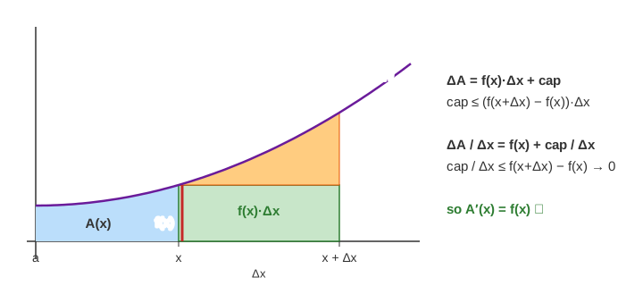
On f = t² at x = 1.5 (f(1.5) = 2.25) the canvas halves Δx twice: ΔA/Δx = 3.0833 at Δx = 0.5, 2.6458 at 0.25 and 2.4427 at 0.125, closing in on 2.25. This is the same limit as on the derivative as a limit page, applied to the area function. (Demo: the sliver, why A′(x) = f(x))
Negative f makes A go down
Area below the axis counts as negative. For f = sin t, A climbs while sin t > 0 and reaches its maximum 2 at x = π, where sin π = 0 and the tangent is flat. On [π, 2π] sin t < 0, each step adds negative area, and A falls back to 0 at 2π: ∫02π sin t dt = 0. The sign of f is the sign of A′, so the zeros of f are the peaks and valleys of A. (Demo: f = sin t, A = 1 − cos x falls where f < 0)
Part 2: evaluate with an antiderivative
A and F have the same derivative f, so they differ by a constant. At x = a, A(a) = 0, so the constant is F(a) and A(x) = F(x) − F(a). Put x = b:
∫ab f(t) dt = A(b) = F(b) − F(a).
For f = t², F(t) = t³/3 gives ∫02 t² dt = 8/3 − 0 = 8/3 ≈ 2.6667. A Riemann sum with 4 midpoint rectangles gives 2.6250 and with 16 gives 2.6641: closer and closer, but only F gives the exact value. Any antiderivative works, because F + C gives (F(b) + C) − (F(a) + C), the same number. (Demo: ∫₀² t² dt = 8/3 via F(t) = t³/3) For how the sums converge, see Riemann sums.
Why it matters
Before the theorem, every area was a limit of sums. After it, integration is "find a function whose derivative is f", which turns the derivative rules (power rule, chain rule, …) backwards into integration rules. It also says that A(x) exists and is differentiable for every continuous f, even when no formula for F is known; then numerical methods like the Riemann and trapezoid sums, or a Taylor series integrated term by term, take over.
Why two antiderivatives differ only by a constant: the Mean Value Theorem (f′ = 0 everywhere means f is constant).
For the intuition first — a tank filling from a rate graph, where the water is the area so far — see Accumulation: rate → amount.
The theorem needs f to be continuous; the three conditions for continuity are animated in Limits & Continuity.
Two techniques for finding antiderivatives, substitution and integration by parts, are drawn as areas on integration by parts and substitution.
Without an antiderivative F, the integral is estimated numerically: Numerical Integration.
What the page leaves out
The proof that a continuous f is integrable, functions with jumps (where A has a corner and A′ ≠ f at the jump), improper integrals with infinite ends, integration techniques (substitution, by parts), the mean value theorem form of the sliver argument, and the multi-dimensional versions (Green's, Stokes' and the divergence theorem).