Critical & Singular Points Visualization

The idea: the slope is zero, or it is missing

A smooth graph looks like a straight line when you zoom in, and the slope of that line is f′(x). Where something interesting happens (a top, a bottom, a pause, a sharp point) the slope is either zero or it does not exist. Points like that are called critical points. The same idea works one level up: on a surface z = f(x, y) the critical points are where the surface is flat, and on a curve F(x, y) = 0 the singular points are where the curve stops being one smooth arc.

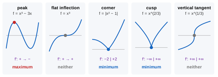
Five small graphs side by side, each with its critical point marked: a peak where f′ goes + then −, a flat inflection where f′ stays +, a corner where f′ jumps from −2 to 2, a cusp where the slope runs to −∞ and +∞, and a vertical tangent where f′ is +∞ on both sides — Five kinds of critical point; only the sign of f′ on the two sides decides peak, valley or neither.

Critical points of f(x)

A number c inside the domain is a critical point of f when f′(c) = 0 or f′(c) does not exist. Fermat's theorem says every peak or valley inside the domain is a critical point, so to find the largest and smallest values you only check the critical points and the two ends. The page slides a tangent along the graph; it turns flat at f′ = 0, and at a missing f′ it breaks into two one-sided tangents or stands up vertically. See the derivative as a limit for why a corner has no derivative.

First-derivative test. Read the sign of f′ just left and just right of c:

f′ left → right	the graph	c is	example on the page
+ → −	rises, then falls	a maximum	x³ − 3x at x = −1, f = 2
− → +	falls, then rises	a minimum	x³ − 3x at x = 1, f = −2; \|x² − 1\| at x = ±1; x^(2/3) at 0
+ → + or − → −	keeps going the same way	neither	x³ at 0 (f′ = 0); x^(1/3) at 0 (no f′)

So a critical point is a candidate, not a verdict: x³ has f′(0) = 0 but only pauses there (Demo: f′ = 0 but no peak). And a missing derivative is no obstacle to being an extreme: |x² − 1| has its two lowest points at corners (Demo: corners, no f′), and x^(2/3) has its lowest point at a cusp (Demo: cusp and vertical tangent). Some books call a point where f′ does not exist a singular point of f, and one where f′ = 0 a stationary point. How the sign of f′ and f″ shapes a graph is on reading f, f′ and f″.

Critical points of f(x, y)

For a surface, the slope is the gradient ∇f = (f_x, f_y). A critical point is where both parts vanish, so on a map it is where the curve f_x = 0 crosses the curve f_y = 0. For f = x³ − 3x − y³ + 3y, f_x = 0 on the lines x = ±1 and f_y = 0 on y = ±1, and they cross at four points (Demo: f(x, y) with four critical points).

Second-derivative test. With D = f_xxf_yy − f_xy² at the point:

D	f_xx	kind	x³ − 3x − y³ + 3y
> 0	< 0	maximum	(−1, 1): D = 36, f = 4
> 0	> 0	minimum	(1, −1): D = 36, f = −4
< 0	any	saddle	(1, 1) and (−1, −1): D = −36, f = 0
= 0	any	the test says nothing	x³ − 3xy² at (0, 0)

At a saddle the surface curves up in one direction and down in another, like a mountain pass. When D = 0 you must look at f itself: x³ − 3xy² is the monkey saddle, with three hills and three valleys around the origin (Demo: monkey saddle, the test fails). On a contour map a top or bottom is a set of closed rings shrinking to a point, and a saddle is where contour lines cross; level curves builds those maps, and gradient descent walks downhill until ∇f ≈ 0.

Singular points of a curve

A curve F(x, y) = 0 is a smooth arc with one tangent near every point where ∇F ≠ 0: this is the implicit function theorem, and ∇F points straight across the curve there. A point of the curve with F_x = F_y = 0 is a singular point, and the curve may do something else there:

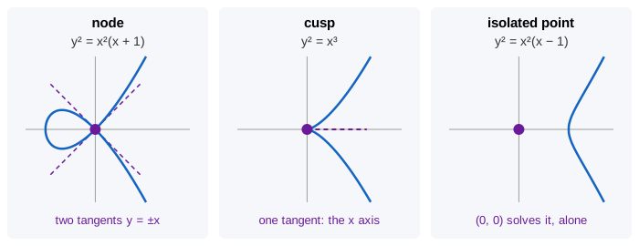
Three curves with their singular point in purple: the node of y² = x²(x + 1) where two branches cross with tangents y = x and y = −x, the cusp of y² = x³ where both halves arrive along the x axis, and the isolated point of y² = x²(x − 1) at the origin, alone to the left of the branch that starts at x = 1 — Node, cusp, isolated point: at all three Fx = Fy = 0, and the curve is not a single smooth arc.

kind	what you see	tangents	example
node	two branches cross	two	y² = x³ − 3x + 2 at (1, 0): y = ±√3(x − 1)
cusp	the curve arrives and turns back	one	y² = x³ at (0, 0)
isolated point	a lone dot, no curve nearby	none	y² = x³ − 3x − 2 at (−1, 0)

On the page a green arrow shows ∇F at points along the curve; it always stands across the curve and shrinks to nothing only at a singular point (Demo: a cusp, y² = x³).

Critical levels: one idea, not two

Every curve y² = x³ − 3x + c is a level curve F = c of the single function F = y² − x³ + 3x. A singular point of the level curve is a point where ∇F = 0, which is exactly a critical point of F. F has two: a minimum at (−1, 0) with F = −2 and a saddle at (1, 0) with F = 2. So the level curves are singular only at c = −2 and c = 2:

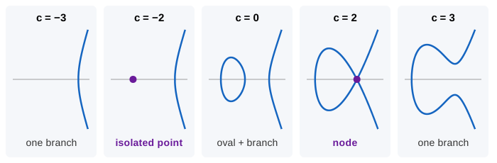
Five panels of y² = x³ − 3x + c for c = −3, −2, 0, 2 and 3: one branch; a branch plus an isolated point at (−1, 0); an oval plus a branch; the oval touching the branch at a node (1, 0); one branch again — The shape changes only at the critical values c = −2 (isolated point, from F's minimum) and c = 2 (node, from F's saddle).

Below −2 there is one branch. At −2 a lone point appears (the bottom of F's bowl), which grows into an oval. At 2 the oval touches the branch and the crossing is a node, because the level through a saddle crosses itself. Above 2 there is one branch again (Demo: y² = x³ − 3x + c as c grows). The same thing happens on the f(x, y) scene: the level f = 0 through both saddles is the line y = x plus the ellipse x² + xy + y² = 3, crossing exactly at the saddles. Studying how level sets change shape only at critical values is the start of Morse theory.

Where it is used

Optimisation is a hunt for critical points: the cheapest design, the best fit of a line to data (least squares sets the gradient to zero), the lowest loss when training a neural network. Physics uses them for equilibria, which are stable at minimum energy and unstable at a saddle. The word "singularity" in complex analysis (a pole such as 1/z at 0) is a different idea: there the function itself is undefined.

The monkey saddle drawn as a 3D surface, with a walk around its three hills and three valleys, is on Monkey Saddle. Surfaces have singular points too: Cayley's nodal cubic has 4 nodes, the Kummer surface has 16, and Surfaces by Degree compares them.

What the page leaves out

Extremes on the boundary of a region and Lagrange multipliers (critical points under a constraint), higher-order tests when D = 0, critical points in three or more variables (the Hessian's eigenvalues), finer kinds of singular point (tacnodes, triple points of higher curves, multiplicity), resolving singular points by blowing up, singularities of complex functions, and singular points of differential equations.