The idea: two markets, one rate, one output
The interest rate depends on output, and output depends on the interest rate. The IS–LM model (John Hicks, 1937, from Keynes's General Theory) solves both at once. The IS curve lists the pairs of rate r and output Y where the goods market clears: what people plan to spend equals what is produced. The LM curve lists the pairs where the money market clears: the money people want to hold equals the money there is. Only where the curves cross are both markets in balance.
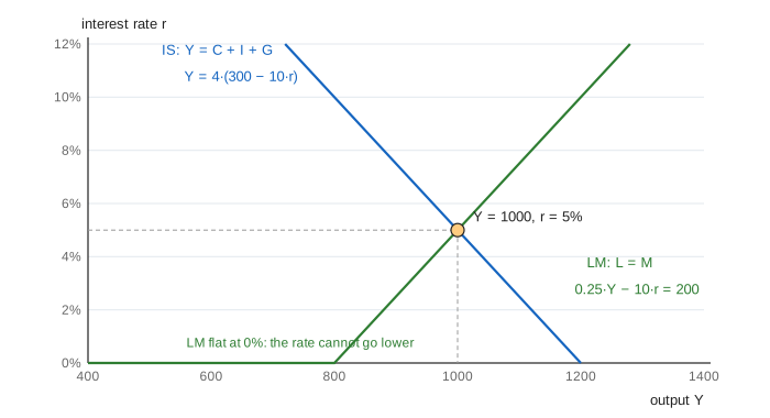
The price level is fixed, so this is a short-run model. The page uses small linear equations you can check by hand:
| Piece | Equation | At the start |
|---|---|---|
| consumption | C = 100 + 0.75·(Y − T) | 775 |
| investment | I = I₀ − 10·r, I₀ = 175 | 125 |
| government, taxes | G = 100, T = 100 | |
| money demand | L = 0.25·Y − 10·r | 200 |
| money supply | M = 200 |
The IS curve: the goods market
Firms produce what people buy, so output settles where Y = C + I + G. Spending feeds on itself. One extra unit of spending is someone's income, and they spend 0.75 of it, which is the next person's income, and so on. The total is the multiplier 1 / (1 − 0.75) = 4. Solving gives Y = 4·(A − 10·r), where A = 100 + I₀ + G − 0.75·T = 300 is the spending that does not depend on income.
A higher rate makes fewer investment projects pay, so I falls and, through the multiplier, Y falls 40 per point. That is why IS slopes down. A change in G, T or confidence (I₀) shifts the whole curve sideways by 4 times the change in A. The "Goods market" panel shows C, I and G as one bar next to output Y.
The LM curve: the money market
People hold money to pay for things, so money demand rises with income: 0.25 per unit of Y. Holding money instead of bonds costs the interest the bonds would pay, so money demand falls as the rate rises: 10 per point. This is Keynes's liquidity preference. The central bank fixes M. Setting L = M gives r = (0.25·Y − M) / 10: more output needs a higher rate to make people part with money, so LM slopes up.
The rate cannot go below zero, because cash always pays 0%. Below Y = M / 0.25 = 800 the curve lies flat on the axis. More money moves LM down and to the right: 5 points lower for each 50 of M.
Fiscal policy and crowding out
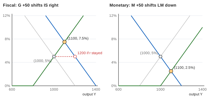
The government buys 50 more (Demo: fiscal expansion, crowding out). At the old rate of 5% the multiplier would take output from 1000 to 1200. But the extra income raises money demand, and with M fixed people sell bonds to get money. Bond prices fall and the rate rises. The higher rate cuts investment from 125 to 100. The new point is Y = 1100, r = 7.5%. Half of the multiplier was crowded out by the higher rate.
Monetary policy
The central bank buys bonds with 50 of new money (Demo: monetary expansion). At the old output, people would hold the extra money only if bonds paid less, so the rate would drop to 0%. The lower rate lifts investment, output rises, and rising output raises money demand again. The rate settles at 2.5% with Y = 1100 and investment at 150.
| Change | Curve | Y | r | I |
|---|---|---|---|---|
| start | 1000 | 5% | 125 | |
| G +50 | IS right | 1100 | 7.5% | 100 |
| M +50 | LM down | 1100 | 2.5% | 150 |
| G +50 and M +50 | both | 1200 | 5% | 125 |
Doing both (Demo: policy mix) keeps the rate at 5%, so nothing is crowded out and output gets the full multiplier: 1200.
The liquidity trap
Firms lose confidence twice (I₀ −50, −50): output falls to 900 and then to 800, and the rate falls to 0%. Now the central bank adds 50 of money (Demo: liquidity trap). Nothing happens. The rate is already zero, no bond pays less than cash, and the extra money sits idle. This is the liquidity trap: Japan after the late 1990s and the US and Europe after 2008.
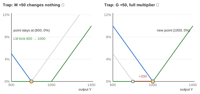
Fiscal policy works best here. G +50 lifts output from 800 to 1000, the full 4 × 50. The rate stays at 0%, because the extra money demand is met from idle money, so nothing is crowded out. A smaller slump (Demo: investment slump, rate cut to zero) shows the limit from the other side: one rate cut brings output back to 1000, but only by using up all the room down to 0%.
From IS–LM to aggregate demand
The model keeps prices fixed. If the price level rises, the same M buys less, so real money falls and LM shifts up: a higher rate and lower output. Plotting output against the price level gives the downward-sloping AD curve of the AD–AS model, which then lets prices move. The circular flow page shows the multiplier as money passing between households and firms.
What the page leaves out
The curves are straight lines and the price level never moves, so there is no inflation and no difference between real and nominal rates. There is no foreign trade or exchange rate (that is the Mundell–Fleming model), no expectations, and one interest rate stands for every rate in the economy. Modern central banks set a rate rather than a quantity of money, so many textbooks now draw LM as a flat line at the policy rate (the IS–MP model). Wealth, debt and the time it takes for policy to work are left out.
See where this page fits on the Economics & Money mind map.