The idea: two ways to store the same edges
Every graph algorithm starts by asking the graph questions: "is u–v an edge?" and "who are the neighbours of u?". How fast those answers come depends on how the graph is stored. There are two classic choices:
- An adjacency matrix: a V × V table. Cell
M[u][v]is 1 ifu–vis an edge, 0 if not. - An adjacency list: one list per vertex.
adj[u]holds the neighbours ofu, and nothing else.
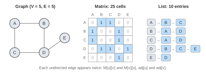
The page stores one undirected graph with 6 vertices both ways and runs every operation on both at once. One step is one read on each side, so the side that needs fewer reads finishes first and waits. The counters under each panel add up the reads.
Memory: V² cells or V + 2E entries
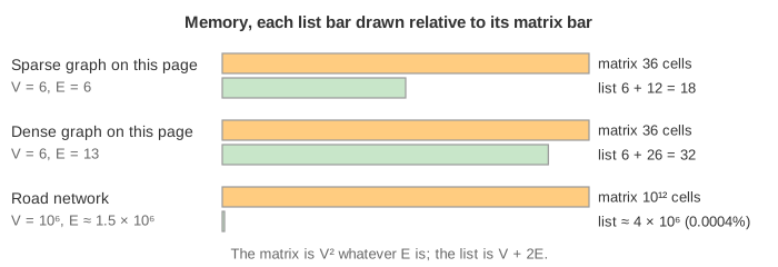
The matrix needs V² cells whatever the edges are: 36 here, with 6 edges or with 13. The list needs V heads plus 2E entries, because an undirected edge u–v is written in adj[u] and in adj[v]. On the sparse graph that is 6 + 12; on the dense graph 6 + 26.
For 6 vertices nobody cares. For real graphs the gap is huge. A road network with a million junctions and about 3 roads each needs V² = 1012 matrix cells (125 GB even at one bit per cell), but only 1 million heads + 2E ≈ 3 million list entries.
What each operation costs
| Operation | Matrix | List |
|---|---|---|
Is u–v an edge? | O(1): read M[u][v] | O(deg u): walk adj[u] |
Neighbours of u | O(V): read the whole row | O(deg u) |
| Add edge | O(1): 2 cells | O(1): append to 2 lists |
| Remove edge | O(1): 2 cells | O(deg u + deg v): find it first |
| Every vertex's neighbours | O(V²) | O(V + E) |
| Memory | V² cells | V + 2E entries |
The matrix wins on edge checks: one cell, no matter how many neighbours u has (Demo 1: is D–E an edge?: 1 cell against 3 list entries, because E is the last entry of adj[D]). The list wins on "neighbours of u": the matrix has to read every 0 in the row too (Demo 2: neighbours of F: 6 cells against 1 entry). Adding is cheap on both; removing from a list needs a scan to find the entry (Demo 5).
Why traversal cost depends on it
BFS, DFS, Dijkstra and Prim all have the same inner loop: take a vertex, then look at each of its neighbours. Over a whole run every vertex is taken once, so the loop reads every vertex's neighbours once.
for each vertex u:            // V times
    for each neighbour v of u:   // matrix: V cells; list: deg(u) entries
        ...
With a matrix that is V × V = O(V²) reads. With a list it is V heads plus the sum of all degrees, which is 2E, so O(V + E). Demo 3 runs this on the sparse graph: 36 cells against 12 entries. Demo 4 runs it on the dense graph: 36 against 26, much closer, because when E is near V²/2 the list has almost as much to read as the matrix.
That is why textbooks write BFS as O(V + E): the bound assumes an adjacency list. With a matrix, the same BFS is O(V²).
Which one to use
- Sparse graph (E much less than V², which covers roads, social networks, the web, dependency graphs): the list. Less memory and traversals in O(V + E).
- Dense graph, or an algorithm that mostly asks "is
u–van edge?": the matrix. Floyd-Warshall works on a V × V matrix anyway. - Small V: either. A matrix of bits fits 64 vertices per machine word and is very fast.
See also BFS vs DFS, which runs the traversal this page counts.
What the page leaves out
- Directed and weighted graphs. A directed edge is written once (
M[u][v]only,adj[u]only); a weight replaces the 1 in the matrix and is stored next to the neighbour in the list. - Linked lists vs arrays for
adj[u], and keeping the lists sorted or in hash sets so edge checks are faster. - Compressed sparse row (CSR): all lists packed into one array plus an offset per vertex, used by graph libraries and GPUs.
- Edge lists (a plain list of pairs), used by Kruskal.
See where this page fits on the Graph Algorithms mind map.