BFS vs DFS Visualization | Queue vs Stack Frontier

The idea: one loop, two frontiers

This page draws one undirected graph twice and runs breadth-first search (BFS) on the left and depth-first search (DFS) on the right, from the same start S, at the same time. Every step visits exactly one new vertex on each side, so the visit numbers (#1, #2, …) and the counters compare the two honestly.

Both searches are the same loop. The vertices that have been seen but not finished form the frontier. Take a vertex from the frontier, look at its neighbours, add the ones not seen yet. The only difference is which vertex comes out next:

BFS keeps the frontier in a queue: first in, first out. The oldest vertex comes out next.
DFS keeps it in a stack: last in, first out. The newest vertex comes out next.

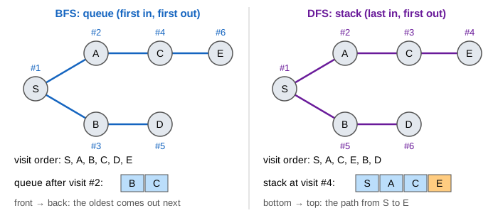
The same small graph twice. BFS with a queue visits S, A, B, C, D, E level by level; DFS with a stack visits S, A, C, E, then backs up to visit B and D — Same graph, same neighbour order: a queue visits ring by ring, a stack goes as deep as it can and then backs up.

Neighbours are always checked in alphabetical order, on both sides, so every run is the same.

BFS: ring by ring, shortest paths

BFS starts with S in its queue. Each step dequeues the vertex at the front, visits it, and enqueues its unseen neighbours at the back, recording the vertex they came from as their parent. Because the queue is first in, first out, every vertex 1 edge from S is visited before any vertex 2 edges away, and so on: BFS visits the graph in rings.

That is why the first time BFS reaches a vertex, the parent pointers give a shortest path, one with the fewest edges. In Demo 1: shortest path BFS reaches G at visit 6 by S→D→G, 2 edges. DFS reaches it at visit 8 by S→A→B→C→F→H→I→G, 7 edges: a path, but not a short one.

queue = [S];  seen[S] = true
while queue not empty:
    u = queue.dequeue()          // visit u
    if u == goal: stop
    for v in neighbours(u):
        if not seen[v]:
            seen[v] = true;  parent[v] = u
            queue.enqueue(v)

DFS: dive, then back up

DFS goes from the current vertex to its first unseen neighbour, then to that vertex's first unseen neighbour, and so on, as deep as it can. When the vertex on top has no unseen neighbour left, DFS pops it and backs up to the vertex below. The page draws recursive DFS, so the stack is the call stack: it always holds exactly the path from S to the current vertex.

dfs(u):
    visit u;  seen[u] = true
    if u == goal: stop
    for v in neighbours(u):
        if not seen[v]:
            parent[v] = u
            dfs(v)

When the goal is at the end of the branch DFS tries first, DFS is fast. In Demo 2 the maze has G at the end of the first corridor: DFS visits S, A, C, E, G, 5 vertices, while BFS must finish every ring closer than G and visits all 12. In Demo 3 the goal is N, at the end of the last corridor. DFS now explores every other corridor to the bottom first and needs 12 visits; BFS needs 11. DFS's speed is luck: it depends on where the goal is and on the neighbour order.

Memory: width vs depth

The frontier is the memory a search needs. BFS's queue holds about one whole ring of the graph, so it grows with the graph's width. DFS's stack holds one path, so it grows with the graph's depth.

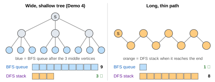
Left: a wide tree, S with 3 children and 9 grandchildren; BFS's queue grows to 9 vertices, DFS's stack to 3. Right: a long path of 8 vertices; BFS's queue never holds more than 1, DFS's stack holds all 8 — A wide, shallow graph fills BFS's queue; a long, thin one fills DFS's stack.

In Demo 4: wide tree BFS's queue grows to 9 (all the leaves at once), and DFS's stack never holds more than 3. The opposite also happens: in Demo 1 DFS walks round the top of the city, and its stack reaches 8 vertices while BFS's queue stays at 3. In a tree with branching factor b and depth d, BFS can hold about b^d vertices, DFS about d (or b·d if it pushes all neighbours at once).

Cycles and non-tree edges

Each search draws a tree: the edges along which it first reached each vertex (blue for BFS, purple for DFS). Any other edge is a non-tree edge. In an undirected graph, a neighbour that is already seen and is not the current vertex's parent means there are two different ways to reach it: the graph has a cycle. The edge turns red.

Both searches can detect a cycle this way, but they find it at different times. In Demo 5 the only cycle is the triangle D, E, F on the first branch. DFS dives into it and sees the back edge F–D after 5 visits; BFS only reaches that depth after finishing the rings before it and sees E–F after 9.

Which one to use

	BFS	DFS
Frontier	queue (FIFO)	stack (LIFO), or recursion
Order	rings of 0, 1, 2 … edges from S	one branch to the bottom, then back up
Shortest path (unweighted)	yes, the first time it reaches the goal	no, any path
Memory	the widest ring, up to `O(V)`	the deepest path, up to `O(V)`
Time	`O(V + E)`	`O(V + E)`
Goal deep down the first branch	slow: all closer rings first	fast
Typical uses	fewest hops, levels, nearest match, web crawl by distance	cycles, topological sort, strongly connected components, mazes, backtracking

You need the path with the fewest edges, or everything within k hops: BFS.
You need to explore everything, find cycles, order dependencies, or the graph is very wide: DFS.
Edges have weights: neither. Use Dijkstra or A*; see them on a grid in Grid Pathfinding.
A huge or infinite graph with a shallow goal: iterative deepening, DFS with a depth limit of 1, 2, 3 …, which gets BFS's shortest path with DFS's small stack.

What the page leaves out

Directed graphs. There a seen vertex is not enough to prove a cycle (two paths can meet without a loop); DFS needs three colours and calls it a cycle only when the edge leads back to a vertex still on the stack.
Iterative DFS that pushes every neighbour at once: it visits vertices in a similar order but its stack can hold b·d entries, some of them seen already.
Bidirectional BFS, which searches from both ends and meets in the middle.
Discovery and finish times, and the edge classes (tree, back, forward, cross) of directed DFS.