The idea: ask the most informative question first
A decision tree classifies a row by asking one question per node: “Outlook?”, then “Humidity?”, until it reaches a leaf that holds the answer. Learning the tree means choosing those questions from a table of labelled examples. The page uses Quinlan's classic play-tennis table: 14 days, four weather attributes, and whether tennis was played (9 Yes, 5 No).
At every node the algorithm tries each attribute, splits the node's rows by its values, and keeps the attribute whose groups are the most pure (mostly one class). Then each group becomes a child node and the same search runs again on fewer rows.
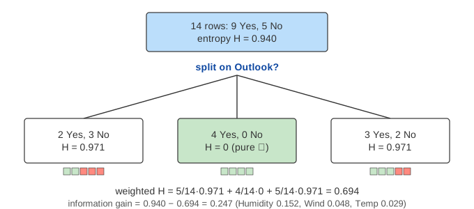
Entropy and information gain
The entropy of a node with class proportions pYes, pNo is H = −Σ p·log₂ p. It is 0 when all rows have the same class and 1 bit for a 50/50 mix. The root has 9 Yes and 5 No, so H = −(9/14)·log₂(9/14) − (5/14)·log₂(5/14) = 0.940.
Splitting on attribute A gives one child per value v. The information gain is the drop in entropy, weighting each child by its share of the rows: gain(A) = H(node) − Σ (nv/n)·H(child v). ID3 picks the attribute with the largest gain.
| Attribute at the root | Rows per value (Yes / No) | Weighted H | Gain |
|---|---|---|---|
| Outlook | Sunny 2/3, Overcast 4/0, Rain 3/2 | 0.694 | 0.247 ✓ |
| Temp | Hot 2/2, Mild 4/2, Cool 3/1 | 0.911 | 0.029 |
| Humidity | High 3/4, Normal 6/1 | 0.788 | 0.152 |
| Wind | Weak 6/2, Strong 3/3 | 0.892 | 0.048 |
The panel under the canvas shows this computation for every node, one attribute per step. (Demo 1: build the ID3 tree)
Gini impurity
CART measures impurity with Gini = 1 − Σ p², the chance that two rows drawn at random from the node have different classes. The root's Gini is 1 − (9/14)² − (5/14)² = 0.459. The best split is the one with the largest Gini decrease; on the root, Outlook again wins (0.116 vs 0.092 for Humidity). Gini needs no logarithm, so it is a little cheaper to compute; it is scikit-learn's default.
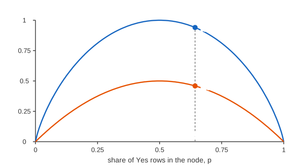
Because the two curves have the same shape, they rank splits almost the same way. On this table both build the identical tree; only the numbers differ. (Demo 3: entropy vs Gini at the root)
Building the tree recursively
After the root splits on Outlook, each child repeats the search on its own rows, without Outlook. The Sunny node (2 Yes, 3 No) finds that Humidity separates it perfectly (gain 0.971); the Rain node finds Wind (gain 0.971). The page processes nodes breadth-first from a queue; real libraries usually recurse depth-first, which gives the same tree.
When a node splits, its rows travel down the branch of their value: the chips D1, D2, … fly from the table to the child nodes. The final tree has 5 leaves and depth 2:
Outlook?
  Sunny    → Humidity?  High → No,  Normal → Yes
  Overcast → Yes
  Rain     → Wind?      Weak → Yes, Strong → No
When to stop
A node becomes a leaf that predicts its majority class when
- it is pure: all its rows have the same class (Overcast: 4 Yes, 0 No);
- it is at max_depth (the root is depth 0);
- no attribute is left on its path, or no split lowers the impurity.
(Demo 2: a pure node stops) Real libraries add more pre-pruning limits:
min_samples_split, min_samples_leaf, min_impurity_decrease.
Overfitting and max_depth
A tree grown until every leaf is pure fits the training rows exactly, including their mistakes. The noisy data adds D15 = Sunny, Cool, Normal, Strong → No: the other Sunny days with Normal humidity are all Yes, so D15 is most likely mislabelled. To make every leaf pure the tree now splits Sunny-Normal on Temp and then Cool on Wind: two extra levels and a rule “Sunny ∧ Normal ∧ Cool ∧ Strong → No” learned from a single row. Its training error is 0, but a new day that looks like D15 gets the noisy answer. (Demo 4: a noisy row grows an overfit branch)
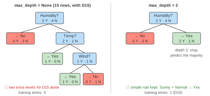
With max_depth = 2 the Sunny-Normal node stops as a leaf with 2 Yes and 1 No, so it
predicts Yes. The tree misclassifies D15 (1 training error) but is back to the simple 5-leaf rule, and the
new day Sunny, Cool, Normal, Strong is classified Yes. (Demo 5: max_depth = 2 stops the overfit)
The right depth is chosen with a held-out validation set or cross-validation, not with training error.
Classifying a new row
Prediction is a walk from the root: at each test node, follow the branch of the new row's value; the leaf's class is the answer. For Sunny, Cool, High, Strong the walk is Outlook = Sunny → Humidity = High → leaf No. It takes at most depth-many comparisons, which is why trees are fast and easy to explain. (Demo 6: classify a new day) If a value never appeared at a node during training, there is no branch, and the page falls back to that node's majority.
ID3, C4.5 and CART
| ID3 (Quinlan 1986) | C4.5 (Quinlan 1993) | CART (Breiman et al. 1984) | |
|---|---|---|---|
| Impurity | entropy, information gain | gain ratio (gain ÷ split information) | Gini (or squared error for regression) |
| Split shape | one branch per value | one branch per value; thresholds for numbers | always binary (value ≤ t, or a subset of categories) |
| Pruning | none | error-based post-pruning | cost-complexity pruning (ccp_alpha) |
Ensembles fix most of a single tree's variance: a random forest averages many trees grown on bootstrap samples with random attribute subsets; gradient boosting adds small trees that each fit the previous ones' errors. See also k-Nearest Neighbors and Naive Bayes, two other classic classifiers, and Gradient Descent, which trees do not need.
Random forests and gradient boosting are animated side by side in Random Forest vs Gradient Boosting.
See also Precision vs Recall for measuring a classifier with a confusion matrix, precision, recall and F1.
What the page leaves out
The page splits categorical attributes into one branch per value for both criteria; real CART (and scikit-learn) makes binary splits and handles numeric attributes with thresholds. Gain ratio, missing values, post-pruning, class weights, regression trees and ensembles are only described. Ties between attributes go to the first column.