Rod cutting: the best way to sell a rod in pieces

The idea: sell the rod in the best pieces

A shop buys long steel rods and sells them cut into pieces of whole inches. A piece of length i sells for the price p[i], and prices are not proportional to length. Given a rod of length n, which cuts earn the most? This is the rod-cutting problem from CLRS §15.1. With the CLRS prices 1, 5, 8, 9 for lengths 1 to 4, a rod of length 4 earns 9 uncut but 10 as two pieces of length 2.

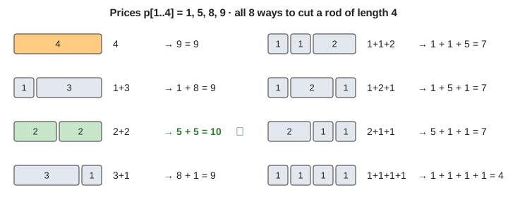
Each of the n − 1 inch marks is either cut or not, so there are 2ⁿ⁻¹ plans. Trying them all is hopeless for long rods, but the plans share their tails, and that is what dynamic programming uses.

The recurrence: first piece plus the best rest

Let r[j] be the most money a rod of length j can bring. Any plan for length j starts with a first piece of some length i (1 ≤ i ≤ j; i = j means no cut). What follows is a rod of length j − i, and in a best plan it must itself be sold the best way, or swapping in a better plan for it would earn more. This is optimal substructure:

r[0] = 0
r[j] = max over 1 ≤ i ≤ j of  p[i] + r[j − i]
cut[j] = the i that gives the max      (ties keep the smallest i)

In the animation the trial rod shows one candidate at a time: the first piece in orange with its price p[i], the rest in blue with r[j − i], read from the table. The side panel lists every candidate and marks the best. (Demo: CLRS prices, n = 4.)

Bottom-up: fill r[0], r[1], …, r[n]

r[j] only reads r[0..j − 1], so filling the row left to right never reads an empty cell. That is CLRS BOTTOM-UP-CUT-ROD; the version that also writes cut[j] is EXTENDED-BOTTOM-UP-CUT-ROD.

r[0] = 0
for j = 1 to n
    best = −∞
    for i = 1 to j
        if p[i] + r[j − i] > best
            best = p[i] + r[j − i];  cut[j] = i
    r[j] = best

With the CLRS prices the row is:

j	0	1	2	3	4	5	6	7	8	9	10
p[j]	–	1	5	8	9	10	17	17	20	24	30
r[j]	0	1	5	8	10	13	17	18	22	25	30
cut[j]	–	1	2	3	2	2	6	1	2	3	10

Rebuilding the cuts from cut[]

r[n] is only the money. To get the pieces, read cut[n]: that is the first piece. Cut it off, and the rest has length n − cut[n], whose first piece is cut[n − cut[n]], and so on until nothing is left. The animation does this on the real rod: each piece appears over the rod, then moves to the pieces row.

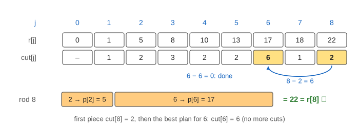
Demo: CLRS prices, n = 7 has a tie: 1 + 6 and 2 + 2 + 3 both earn 18. The strict ">" keeps the first candidate, i = 1, so the page shows 1 + 6. Demo: n = 10 ends with cut[10] = 10: the uncut rod, worth 30, beats every cut.

Greedy by price per inch fails

A natural shortcut is to cut first the piece with the best density p[i] / i, then repeat on the rest. With the CLRS prices and n = 4 the best density is length 3 (8 / 3 ≈ 2.67), so greedy sells 3 + 1 for 9, not 10. Demo: greedy by price per inch fails makes the gap bigger: prices 1, 2, 15, 21, 22, 24 and n = 6. Length 4 has the best density (21 / 4 = 5.25), but it leaves 2 inches worth only 2, so greedy gets 23 while 3 + 3 earns 30. Grabbing the best-looking piece can spoil the rest, so every first piece has to be tried.

The unbounded-knapsack pattern

Rod cutting is an unbounded knapsack: the rod length is the capacity, a piece of length i is an item of weight i and value p[i], and each piece length can be used any number of times. The table is one row indexed by capacity, and each cell tries every item as "the first one". The 0/1 knapsack differs only in that each item is used at most once, which needs a second index for "items considered so far". Coin change is the same pattern with coins instead of pieces.

problem	capacity	items	each item	cell
rod cutting	rod length j	piece lengths 1..n	any number of times	max p[i] + r[j − i]
unbounded knapsack	weight w	items	any number of times	max vi + best[w − wi]
0/1 knapsack	weight w	items 1..i	at most once	max of skip, vi + best[i − 1][w − wi]

Running time

Filling r[j] checks j candidates, so the whole row needs 1 + 2 + … + n = n(n + 1)/2 checks: Θ(n²) time and Θ(n) space for r[] and cut[]. For n = 10 that is 55 checks against 2⁹ = 512 plans; for n = 40 it is 820 checks against more than half a trillion plans. The plain recursive CUT-ROD, without a table, solves the same small rods again and again and takes 2ⁿ calls; see memoization vs tabulation for that difference on a smaller example.

What the page leaves out

Rods are capped at 10 inches so the row fits on the canvas. The page leaves out the memoized top-down MEMOIZED-CUT-ROD (same table, filled on demand), a fixed cost per cut (CLRS exercise 15.1-3), a limit on how many pieces of each length can be sold, and the subproblem graph view of the recurrence.

References

Cormen, Leiserson, Rivest, Stein: Introduction to Algorithms, §15.1 Rod cutting (3rd ed.; §14.1 in the 4th ed.)

Cutting stock problem (Wikipedia)

Unbounded knapsack problem (Wikipedia)