The idea: two roads from human preferences to a better model
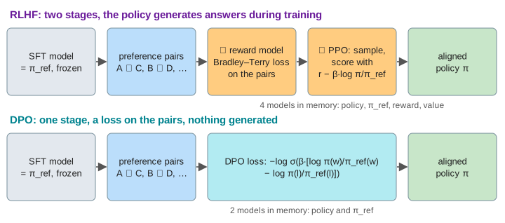
A pretrained and instruction-tuned (SFT) model already writes plausible answers, but not always the ones people want. To fix that, people compare pairs of answers and say which one is better. Two methods turn those preference pairs into a better model. RLHF (reinforcement learning from human feedback) first trains a reward model on the pairs, then improves the model with the reinforcement-learning algorithm PPO. DPO (direct preference optimization) trains the model on the pairs directly with one loss. The page runs both on the same toy model and the same pairs, side by side.
The toy model and the data
The prompt is “How do I undo my last git commit?” and the model can give four answers, A to D. The policy π is just a probability for each answer (a softmax over four numbers). The SFT model is kept, frozen, as the reference π_ref = (0.20, 0.25, 0.30, 0.25). It likes the harmful answer C, “rm -rf .git”, best. A real LLM has the same structure, only its “answers” are every possible token sequence, as on How a Large Language Model Works.
The human data is three pairs with 10 votes each: A ≻ C 9:1, B ≻ D 8:2 and A ≻ B 6:4. The labelers do not always agree, and both methods use the vote share q (0.9, 0.8, 0.6), not just the winner.
RLHF stage 1: the reward model
The reward model gives each answer a score r(y). The Bradley–Terry model says a person prefers w over l with probability σ(r(w) − r(l)), so training minimises −log σ(r_w − r_l) over the pairs, a logistic regression on score differences (the same loss as on Softmax & Cross-Entropy). After two rounds the scores are A 1.10, B 0.69, C −1.09, D −0.70 and the loss has gone from 0.693 to 0.500. It cannot reach 0: with 9:1 votes the best a model can do is predict 0.9. (Demo: RLHF — reward model, then PPO)
RLHF stage 2: PPO with a KL penalty
Now the policy learns. Each round it writes 256 answers from its current probabilities, the reward model scores them, and answers that scored above the batch average become more likely. This is the reinforcement-learning loop of Q-Learning, with the reward model as the environment. Left alone, the policy would pile all its probability on the top-scoring answer and could drift into text the reward model has never seen and scores wrongly (reward hacking). So every score gets a penalty:
R(y) = r(y) − β · log( π(y) / π_ref(y) )
Averaged over the samples the penalty is the KL divergence KL(π‖π_ref), how far the policy has moved from the reference. PPO also clips each update: an answer's probability may change by at most ×1.2 (ε = 0.2) per round. After 8 PPO rounds at β = 0.5, π(A) has gone from 0.20 to 0.61 and π(C) from 0.30 to 0.04.
DPO: the reward model hidden in the policy
The RLHF objective, reward minus β·KL, has a known best answer: π*(y) = π_ref(y) · exp(r(y)/β) / Z. DPO turns this around and writes the reward in terms of the policy, then puts it into the Bradley–Terry loss. The normaliser Z, a sum over every possible answer that nobody can compute for a real LLM, cancels out.
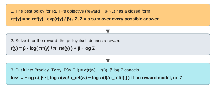
The result is one loss on the pairs, −log σ(β · [log π(w)/π_ref(w) − log π(l)/π_ref(l)]). It only needs the policy's and the reference's probabilities for answers that are already in the data: no reward model, no sampling, no PPO. The quantity β·log(π/π_ref) is the implicit reward, shown in the DPO lane's right column. After 4 rounds π(A) is 0.63, π(C) 0.02. (Demo: DPO — one loss on the same pairs)
Same data, same target
Both methods aim at the same π*, drawn as a dark tick on every bar. At β = 0.5 the target is π*(A) = 0.62; RLHF ends at 0.61 and DPO at 0.63. The reward model says r(A) − r(C) = 2.19; DPO's implicit reward gives 2.06 without ever building a reward model. (Demo: side by side — both reach the same policy)
| β | target π*(A) | RLHF π(A), KL | DPO π(A), KL |
|---|---|---|---|
| 0.1 | 0.98 | 0.86, 1.06 (still climbing) | 0.98, 1.52 |
| 0.5 | 0.62 | 0.61, 0.61 | 0.63, 0.72 |
| 1 | 0.45 | 0.46, 0.33 | 0.45, 0.31 |
β: how long the leash is
β weighs the KL penalty in both methods. With β = 0.1 the leash is loose: the target puts 98 % on A and moves far from the reference (KL 1.5). DPO gets there in 4 rounds; RLHF is still at 0.86 after 8 PPO rounds, because the clip lets each probability grow only ×1.2 per round. (Demo: β = 0.1) With β = 1 the leash is tight: A only rises to 0.45 and the harmful answer C keeps 8 %. (Demo: β = 1) Real runs use β around 0.01 to 0.5 and watch the KL during training.
Cost and when to pick which
| RLHF (reward model + PPO) | DPO | |
|---|---|---|
| stages | 2: fit the reward model, then RL | 1 |
| models in memory | 4: policy, reference, reward model, value model | 2: policy and reference |
| generates text while training | yes, every PPO round | no, only reads the dataset |
| hyperparameters | many (β, clip ε, learning rates, batch, value loss) | few (β, learning rate) |
| strength | learns from its own fresh samples; the reward model can score new prompts and answers | simple, stable, cheap; behaves like supervised fine-tuning |
| weakness | expensive and fiddly; reward hacking | only sees answers in the data; can overfit when one side always wins |
Small trainable add-ons such as LoRA are often used for both, and with LoRA the reference model is just the base weights with the adapter switched off.
The PPO step of RLHF is a policy-gradient update with a learned critic, shown from scratch in Policy Gradient: REINFORCE.
What the page leaves out
A real policy is a transformer over token sequences, not four fixed answers, so its log-probabilities are sums over tokens and the KL penalty is usually applied per token. Real PPO has a learned value model and GAE advantages; the page uses the batch average as the baseline, which is closer to RLOO or GRPO. The reward model is a full network that generalises to new answers, which is what makes reward hacking possible. The page also leaves out the SFT stage itself, variants such as IPO, KTO, ORPO and online or iterative DPO, and constitutional AI, where an AI model writes the preference labels.