The idea: put the keys you look for most near the root
A search in a binary search tree compares the key with one node per level, so finding a key at depth d costs d comparisons (the root has depth 1). A balanced tree keeps every depth small, which is the best you can do when you know nothing about the searches. But if you know how often each key is searched, its frequency, you can do better: put the hot keys near the root, even if the tree becomes lopsided. The optimal binary search tree is the tree with the fewest comparisons in total. The page finds it with dynamic programming over ranges of keys.
The cost of a tree
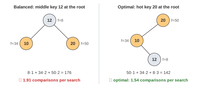
Number the sorted keys k1 < k2 < … < kn and let f(i) be how many searches ask for ki. The cost of a tree is the total number of comparisons, Σ f(i) · depth(ki). Divided by the number of searches W = f(1) + … + f(n), it is the expected number of comparisons per search. For keys 10, 12, 20 with frequencies 34, 8, 50 the balanced tree costs 176 and the tree rooted at 20 costs 142. (Demo: 3 keys 10, 12, 20)
Trying every tree is hopeless for many keys: n keys have Cn different binary search trees (the Catalan numbers again: 5 for 3 keys, 42 for 5 keys, 16,796 for 10 keys).
The recurrence: try every root
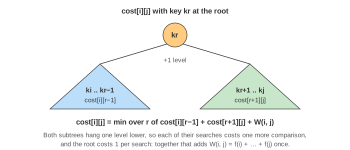
Some key kr is the root. Then keys ki..kr−1 form the left subtree and kr+1..kj the right subtree, and each subtree must itself be the best tree for its keys, or swapping in a better one would improve the whole tree (optimal substructure). Hanging both subtrees under the root moves each of their keys one level down, and the root itself costs one comparison per search. So the root adds exactly W(i, j) = f(i) + … + f(j), whichever key it is:
cost[i][i−1] = 0, cost[i][j] = min over i ≤ r ≤ j of cost[i][r−1] + cost[r+1][j] + W(i, j)
The root table root[i][j] stores the r that gave the minimum. On the canvas the candidate list shows every r for the cell being filled; the blue and green cells are the two subtrees of the winner, and the key boxes on top are coloured the same way, with the root in orange.
Filling by range length, then the trace back
A cell reads only cells for shorter ranges, so the table is filled by length j − i + 1, exactly like matrix chain multiplication: first the diagonal, cost[i][i] = f(i) (a single key is a root at depth 1), then all ranges of two keys, and so on up to cost[1][n], the answer. To build the tree, start at root[1][n], make that key the root, and look up the root of each side in the same table. On the canvas each Step of the trace back adds one node. At the end the tree's Σ f·depth is written out term by term and equals cost[1][n].
When two roots give the same cost the page keeps the one nearest the middle of the range. With equal frequencies that gives exactly the balanced tree. (Demo: equal frequencies give the balanced tree)
Balanced and greedy trees are not optimal
Two simple rules compete with the table. Balanced: put the middle key at the root. It ignores the frequencies. Greedy: put the most frequent key at the root, then repeat on each side. It ignores how the root splits the rest: with frequencies 15, 10, 5, 10, 20 greedy puts 50 at the root and leaves four keys on one side, while the optimum puts 20 at the root and splits the rest. (Demo: 5 keys, most frequent at the root is not best) With one very hot key the optimum is a lopsided, almost chain-like tree, and the balanced tree needs half as many comparisons again. (Demo: one hot key, skewed frequencies)
| keys : frequencies | optimal | balanced | greedy |
|---|---|---|---|
| 10:34, 12:8, 20:50 | 142 | 176 | 142 |
| 10:80, 20:10, 30:5, 40:3, 50:2 | 137 | 207 | 137 |
| 10:10, 20:10, 30:10, 40:10, 50:10 | 110 | 110 | 150 |
| 10:15, 20:10, 30:5, 40:10, 50:20 | 130 | 145 | 145 |
Running time and space
There are n(n + 1)/2 cells, and a cell for a range of length l tries l roots, so the table takes Θ(n³) time and Θ(n²) space: 35 root checks for 5 keys instead of 42 whole trees. Knuth showed that the best root moves monotonically, root[i][j−1] ≤ root[i][j] ≤ root[i+1][j], which cuts the time to Θ(n²). The same interval-DP shape solves matrix chain multiplication.
See also Binary Search Tree for how search, insert and delete work on one tree, and Matrix Chain Multiplication for the same table filled by length with a split in the middle.
What the page leaves out
Only successful searches are counted. The CLRS version also has dummy keys d0..dn for searches that fall between keys and miss, with their own probabilities q; they add q terms to W and change the diagonal, but the recurrence and the table are the same. The page is also capped at 5 keys and leaves out Knuth's O(n²) speedup, the memoized top-down version, and self-adjusting trees such as splay trees, which approach the optimum without knowing the frequencies in advance.
See where this page fits on the Dynamic Programming mind map.