MariaDB: How the Optimizer Picks a Join Order

The idea: grow a left-deep plan one table at a time

A query that joins n tables can run them in n! orders. The optimizer has to pick one before it reads any row. MariaDB only builds left-deep plans: a prefix of tables that is already joined, plus one more base table on the right. So it can describe every plan as an order like D, P, W, E and grow it one table at a time.

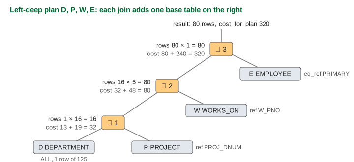
The page uses four tables from the book's COMPANY schema: DEPARTMENT D (125 rows, 13 blocks, the book's numbers), EMPLOYEE E (10,000 rows, 2,000 blocks), PROJECT P (2,000 rows) and WORKS_ON W (10,000 rows). The query keeps one department, D.Dname = 'Dept5', and has four join conditions, one per edge of the join graph on the canvas.

SELECT E.Lname, P.Pname
FROM DEPARTMENT D, EMPLOYEE E, PROJECT P, WORKS_ON W
WHERE D.Dname = 'Dept5' AND E.Dno = D.Dnumber AND P.Dnum = D.Dnumber
  AND W.Pno = P.Pnumber AND W.Essn = E.Ssn;

Pricing one step: rows x fanout

Adding table T to a prefix that outputs r rows gives r x fanout rows. The fanout is how many rows of T match one prefix row. It comes from the book's join selectivity, js = 1 / max(NDV(A), NDV(B)): fanout = |T| x js. For E.Dno = D.Dnumber, js = 1/125 and the fanout is 10,000 / 125 = 80. If no condition links T to the prefix, the fanout is all of |T|: a Cartesian product.

The cost of the step depends on r, not on the result. MariaDB takes the cheaper of two ways to reach T:

Access (EXPLAIN type)	Cost on the page	Book formula
ref / eq_ref: one index lookup per prefix row	r x (x + 1 + s), or r x (x + 1) for a key or covering index	J2 index nested loop
ALL + join buffer (BNL)	blocks(T) once per 1,000 buffered prefix rows	J1 nested loop with buffers

So [D] + E costs 1 x 83 (EMP_DNO: 2 index levels + 1 + 80 rows), but [D,P] + E costs 16 x 83 = 1,328, because 16 rows now come out of the prefix. Small intermediate results make every later step cheap. Demo 2: price the winner D,P,W,E walks through it; Demo 3: Cartesian product D,W,P,E shows 10,000 rows appearing after the second table and the cost growing to 25,513.

The depth-first search and pruned_by_cost

MariaDB does not price all 24 orders. Its function best_extension_by_limited_search() extends the prefix depth first. At each level it tries the candidates with the fewest rows first. The first complete plan becomes the best plan. After that, any partial plan whose cost is already at least the best cost is cut (pruned_by_cost in the optimizer trace): adding tables can only add cost, so none of the orders below it can win.

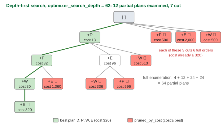
The first plan found is cheap because the search starts with the most selective table, D (1 row). That is what makes pruning work. Demo 1: exhaustive search, depth 62 runs it: 12 partial plans, 7 of them pruned_by_cost, best order D, P, W, E. On MariaDB 13.1, with tables built to these sizes, the optimizer trace lists the same 12 entries in the same order, with the same rows, and EXPLAIN shows the same plan: D ALL, P ref PROJ_DNUM, W ref W_PNO (Using index), E eq_ref PRIMARY.

optimizer_search_depth: greedy search for big joins

A full depth-first search still grows like n!. The variable optimizer_search_depth (default 62, 0 = let the server choose) limits how many tables ahead the search looks. If it is at least the number of tables, the search is exhaustive. If it is smaller, greedy_search() runs a search d tables ahead, keeps only the first table of the best extension, and searches again from the longer prefix.

optimizer_search_depth (MariaDB 13.1 trace)	Partial plans examined	pruned_by_cost	Order
62 (exhaustive)	12	7	D, P, W, E
2 (two tables ahead)	15	9	D, P, W, E
1 (pure greedy)	10	6	D, P, W, E

With 4 tables the greedy searches find the same order; depth 2 even examines more, because it searches again from each fixed prefix. With 20 tables the difference is huge, and a small depth can miss the best order. (Demo 4: pure greedy, depth 1, Demo 5: look 2 tables ahead, depth 2.)

optimizer_prune_level

optimizer_prune_level adds heuristic cuts on top of pruned_by_cost. At level 1 a candidate is dropped (pruned_by_heuristic) when, roughly, a sibling already tried at the same level has both fewer rows and a lower cost. Level 2, the default since MariaDB 10.10, also joins tables reached through eq_ref as one unit instead of trying them in every position. Level 0 turns the heuristics off. In this 4-table query the heuristics never fire: the MariaDB 13.1 trace shows the same 12 entries at levels 0, 1 and 2.

The join algorithm of each step

While it prices a step, MariaDB also picks how to run it. Every step is a nested loop over the prefix rows. The inner table is reached through an index (ref, eq_ref) or through the join buffer, which join_cache_level (default 2) controls: 1–2 block nested loop (BNL, flat or incremental), 3–4 BNLH (a hash table built over the buffered rows), 5–8 batched key access (BKA, BKAH), which sorts the lookup keys before going to the index. EXPLAIN shows it as Using join buffer (flat, BNL join). The page only uses ref, eq_ref and BNL. Join Algorithms animates nested loop and hash join.

Reading it in the optimizer trace

SET optimizer_trace = 'enabled=on';
SELECT ...;   -- the query above
SELECT trace FROM information_schema.OPTIMIZER_TRACE;

Under considered_execution_plans each entry has a plan_prefix, the table being added, rows_for_plan and cost_for_plan, and pruned_by_cost: true when it is cut. The chosen order is best_join_order. The search tree on the canvas lists the same entries in the same order. MariaDB's cost units are not block reads, but the pattern of cuts is the same.

See also How a Query Planner Picks a Plan (PostgreSQL's planner, which uses dynamic programming), MySQL JOIN, GROUP BY and ORDER BY and Database Indexes.

What the page leaves out

Real costs are MariaDB's own units (index and row reads, a per-row WHERE cost, the optimizer_*_cost variables of MariaDB 11), not block reads. Rows count only the join condition used for the lookup, as in the real trace (rows_for_plan stays 80 after E even though E.Dno = D.Dnumber also filters); optimizer_use_condition_selectivity and histograms refine local filters. Semi-join strategies, outer joins, constant tables found before the search and STRAIGHT_JOIN are left out. The book's sort-merge join is left out because MariaDB has none. Bushy and right-deep trees are left out because MariaDB only builds left-deep plans. The book's dynamic programming over subsets is left out because MariaDB searches depth first instead.

References

MariaDB: optimizer_search_depth, optimizer_prune_level, join_cache_level

MariaDB: Block-based join algorithms (BNL, BNLH, BKA)

MariaDB: Optimizer trace overview

Elmasri & Navathe, Fundamentals of Database Systems, 7th ed., Section 19.5: cost functions for JOIN, join selectivity, join ordering.