The idea: cut the space, or wrap the points
A map app asks: which point is closest to me? and which points are inside this box? Checking every point works for 15 points, not for 15 million. A spatial index groups the points by where they are, so a search can skip whole regions at once. This page builds two classic ones on the same 15 points A–O: a KD-tree and an R-tree.
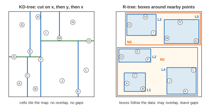
The map is a 64 × 64 square. Pick the index with the index select, and a query point q with the query select.
KD-tree: split at the median, x then y
A KD-tree (k-dimensional tree) is a binary search tree whose key changes with the depth. At depth 0 it compares x, at depth 1 y, at depth 2 x again. Each node holds one point and draws a line through it across its cell: smaller values go left, larger go right.
- To build a balanced tree, sort the cell's points on the current axis and take the median. Half the points go to each side.
- The root is F (24, 28) with the line x = 24. The left half splits at D, y = 30; the right half at O, y = 42.
15 points give a perfect tree: 15 nodes in 4 levels, 7 lines and 8 leaf cells (Demo: KD-tree build). The cells cover the map with no overlap and no gaps.
Nearest neighbour: go down, then back up
The search first goes down the side of each line where q lies, like a lookup in a binary tree. Every point it passes is a candidate; the closest one so far is the best, drawn as an orange circle around q.
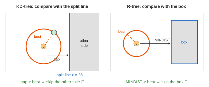
The first leaf is only a guess. On the way back up, each node asks: is q closer to my line than the best distance? If yes, the circle crosses the line, and the other side may hold a closer point, so it is searched too (backtracking). If not, the whole other side is skipped: it is pruned.
For q (32, 46): the search goes F → O → M → I and finds I at 4.5. Back at M, q is 6 from x = 38: skip. Back at O, q is only 4 from y = 42, less than 4.5: search K and J (no better). Back at F, q is 8 from x = 24: skip 7 points. It checks 6 of 15 points (Demo: KD-tree nearest neighbour).
R-tree: boxes around nearby points
An R-tree stores, in every node, up to M entries (here M = 3). A leaf holds points; an inner node holds child nodes. Each node keeps the minimum bounding rectangle (MBR) of everything below it: the smallest box that covers it.
This page loads all points at once with STR (Sort-Tile-Recursive):
- 15 points need P = ⌈15 / 3⌉ = 5 leaves. Sort by x and cut slices of S · M = 9 points, with S = ⌈√5⌉ = 3. That gives a western slice of 9 and an eastern slice of 6.
- Sort each slice by y and pack each run of 3 into a leaf: L1 = A B C, L2 = D E F, L3 = G H I, L4 = J K L, L5 = M N O.
- Do the same with the 5 leaf boxes: N1 = L1 L2 L4 (the south), N2 = L3 L5 (the north). The 2 boxes left fit in the root. Height 3 (Demo: R-tree build).
Unlike KD-tree cells, boxes can leave empty space between them, and in general they can overlap. A point is in exactly one leaf, but a query may have to look into several boxes that cover the same spot.
Nearest neighbour in an R-tree: MINDIST
MINDIST is the distance from q to the closest edge of a box, or 0 if q is inside it. No point in the box can be closer than that. The search opens the child boxes in MINDIST order and skips every box whose MINDIST is not smaller than the best distance so far.
For q (32, 46): the root's boxes are N2 at 0 and N1 at 12. In N2, L3 is 4.5 away and L5 6.0. L3's points give I at 4.5. Then L5 (6.0) and N1 (12.0) are both skipped. It opens 3 nodes and checks only 3 points (Demo: R-tree nearest neighbour).
Range search
A range search finds every point inside a box, here 24 × 20 around q. The KD-tree skips a side of a line when the box lies wholly on the other side. The R-tree opens only the children whose box intersects the query box.
For q (32, 46) the box is x 20–44, y 36–56, and both find I and M. The KD-tree checks 10 points (the line x = 24 passes through the box, so both halves of the map are searched). The R-tree skips N1 at once and checks 6 (Demos: KD-tree range search, R-tree range search).
Which one checks fewer points?
It depends on the data and the query. For q (32, 46) the R-tree checks 3 points and the KD-tree 6. For q (12, 44) the KD-tree checks 5 and the R-tree 6, because N1 is 10.0 away, just under the best distance 10.2, so the R-tree must open it too and check L2 for nothing (Demo: same query on both trees).
| KD-tree | R-tree | |
|---|---|---|
| Divides | The space, with lines through points | The data, with boxes around groups |
| Node holds | 1 point and 1 split | Up to M boxes or points (M is often 50–200, one disk page) |
| Regions | Never overlap, no gaps | Can overlap, can leave gaps |
| Indexes | Points | Points and shapes (lines, polygons) by their boxes |
| Inserts and deletes | Easy, but the tree gets unbalanced; often rebuilt | Stays balanced like a B-tree: nodes split when full |
| Typical home | In memory: nearest-neighbour search, point clouds, ML | On disk: spatial indexes in databases |
Where they are used
R-trees are the spatial index of databases: PostGIS builds an R-tree over GiST, SQLite has an R*Tree module, and MySQL InnoDB uses R-trees for SPATIAL INDEX. KD-trees are common in memory: scikit-learn's KDTree and its k-nearest neighbours classifier, nanoflann and FLANN, and point-cloud libraries such as PCL.
See also quadtree vs geohash, which cut the map into four quarters or a fixed grid instead; binary search trees, the one-dimensional KD-tree; and B-trees, whose node splits an R-tree copies when it inserts one point at a time.
What the page leaves out
Inserting into an R-tree one point at a time (Guttman's ChooseLeaf by least enlargement, and the linear or quadratic split of a full node), the R*-tree's forced reinsert, and deletes. Best-first nearest-neighbour search with a priority queue, and k nearest neighbours instead of one. KD-trees in more than 2 dimensions, where pruning gets weak (the curse of dimensionality), and variants that keep points only in leaves. Real maps also need distances on a sphere.